PRECIPITATION GAUGE NETWORK - PowerPoint Presentation

Slide1

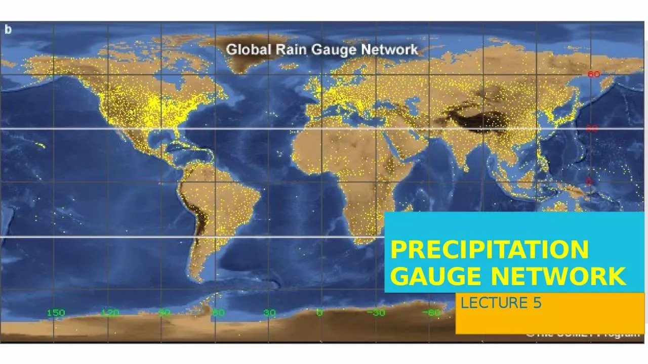
PRECIPITATION GAUGE NETWORK

LECTURE 5

Slide2

PRECIPITATION GAUGE NETWORK

To have an idea of areal distribution of precipitation there should be adequately planned rain gauge networkThere are two reasons to plan a network:

Catch area of a precipitation gauge is very small

Amount of precipitation varies from place to place

Slide3

PRECIPITATION GAUGE NETWORK IN PAKISTAN

Slide4

GAUGE DENSITY (G.D)

On average basis the area served by one rain gauge is called gauge density. G.D =

Lesser value of G.D means more no. of rain gauges in the area which are closely spaced and vice-versa

World Meteorological Organization (W.M.O) has recommended certain gauge densities

 

Slide5

W.M.O RECOMMENDED GAUGE DENSITIES

For Flat regions 600-900 Km2

/station

For mountainous regions 100-250 Km

2

/station

For small mountainous islands 25

Km

2 /stationFor arid and polar zones 1500-10,000 Km2 /station

Slide6

FACTORS AFFECTING GAUGE DENSITY

TopographyFor hilly terrains G.D should be lesser because generally more rains and more variations

Hydro-meteorology

Areas with more precipitation should have less G.D

Stream network

Denser stream network lesser will be G.D

Population density

More population lesser should be G.D

EconomyLesser G.D.P more G.DInterestClimatological station is must on airports and water control reservoirsResearchLesser G.D results in better output

Slide7

INTERPRETATION OF PRECIPITATION DATA FROM A GAUGE NETWORK

Interpretation of rain data coming from a rain gauge network includes

Estimation of missing precipitation data

Checking consistency in precipitation data record

Determination of average areal precipitation

Slide8

1.ESTIMATION OF MISSING PRECIPITATION DATA

According to US environmental data services, for estimation of missing precipitation record, there should be atleast three surrounding stations (Index Stations)

Index stations should be having more or less same effective radii as station “X

” (station for which precipitation data is missing)

And these stations should be more or less equally spaced around station “X”

X

B

C

A

Slide9

1.ESTIMATION OF MISSING PRECIPITATION DATA

There are two methods for estimation of missing precipitation based on Normal Annual Precipitation (N.A.P)

Arithmetic mean method

Normal ratio method

Normal Annual Precipitation : mean of annual precipitation of 30 years record is called normal annual

precipitation.

NAP=

 

X

B

C

A

Slide10

a)ARITHMETIC MEAN METHOD

NAP of the index stations are within 10% of the station at which precipitation data is missingMissing data then can be estimated by simple arithmetic average of the precipitation of that day or the year at index stations

P

x

=

P

x

: Missing precipitation at station X

P

A

,

P

B

,P

C

=Precipitations at index stations at same time

 

X

B

C

A

Slide11

b)NORMAL RATIO METHOD

When normal annual precipitation of station “X” differs more than 10% from any of the index stations then missing precipitation is assessed by this methodIn this method amount of precipitation is weighted by the ratios of normal annual precipitation values.

P

x

=

P

A

+

P

B

+

P

C

]

P

x

=

+ + ]Px

: Missing precipitation at station X

PA , P

B ,PC

: Precipitations at index stations at same time

NX : normal annual precipitation at station X

NA ,

NB

,

N

C

:

normal annual

precipitations

at index stations

 

X

B

C

A

Slide12

NUMERICAL PROBLEM

Precipitation station X was inoperative on 24 august, 2010. The precipitation records for the same date at three surrounding stations A,B and C were 82,87 and 97mm respectively. Normal Annual Precipitations at station X, A,B and C are 920,800,810 and 950mm respectively

Slide13

NUMERICAL PROBLEM

Solution:Which method is to be used? Based on NAP

10% of NAP at Station X (N

X

) = 92

N

X

+10% = 1012mm and N

X -10% = 828mmFor arithmetic method NA , NB and NC should lie between (1012-828)Which is untrue for this case.Apply Normal Ratio Method and determine missing precipitation for the date mentioned

P

x

=

+

+

] PX = 95.68 mm  

Slide14

2. CONSISTENCY OF PRECIPITATION RECORD

Double mass analysis tests the consistency of the record at a station by comparing its accumulated annual or seasonal precipitation with concurrent accumulated values of mean precipitation for a group of surrounding stationsA change in the slope indicates a change in precipitation regime at station.

Any change due to meteorological reasons will not cause change in slope because all the base stations and the station whose consistency is in question will be affected equally

Slide15

DOUBLE MASS CURVE

Slide16

DOUBLE MASS CURVE

If change in slope occurs the year of change is determined using double mass curve and station history is seen for any important event in that year.Conditions before and after change year are assessed and data is adjusted according to reliable data.

Adjustment is made by using ratio of the slopes of the lines before and after change

Adjustment factor =k=

 

Slide17

DOUBLE MASS CURVE

Number of surrounding stations should be atleast 10

Considerable caution must be exercised in applying this

technique.

Because the plotted points deviate about a mean line and changes in slope should be only accepted if there is a marked difference substantiated by other evidences too.

If the slope change remains for a period less than 5 years this change is ignored. Data is considered consistent

Depending upon conditions any of the data before or after the change year may be reliable but generally latest data is taken as reliable.

Slide18

CAUSES OF INCONSISTENCY

Change in the location e.g., gauge near a river siteChange in the instrument e.g., modern, better performanceChange in observational procedures

Slide19

3. AVERAGING PRECIPITATION OVER AN AREA

Average depth of precipitation over a specific area on a storm, seasonal or annual basis is required in many types of hydrologic problems.This average depth when multiplied with the area under consideration provides total volume of water generated in a storm, or seasonally or annually.

There are mainly three methods to compute average depth

Arithmetic average

Thissen’s method

Isohyetal method

Slide20

a) ARITHMETIC AVERAGE METHOD

Simplest method of obtaining average depth over an area is arithmetic mean of the gauges present in the areaThis technique yields good estimated in flat countries where the gauges are more or less uniformly spaced

And individual gauge catches do not vary much from the mean value

These limitations can be partially overcome if topographical influences and areal representation are considered while installing gauges

Slide21

a) ARITHMETIC AVERAGE METHOD

Applicability: Uniform precipitation almost at all stations

Stations are equally spaced in the area

For very small and plane areas results may be satisfactory

Merits:

This is a quick and simple method

Demerits

:

When there is variation in precipitation almost 10% from the mean value outcome is not very true. Also not applicable to areas with unequal spacing between stations. These are generally most encountered conditions

Slide22

b) THE THISSEN’S METHOD

This method attempts to allow for non-uniform distribution of gauges by providing a weighing factor for each gaugeStations are plotted on a map and connecting lines are drawnPerpendicular bisectors are marked and by their intersection polygons are made. Each polygon is effective area for that gauge.

Area of each gauge is determined then by

planimetry

and is presented as percentage of total area

Weighted average rainfall for the total area is computed by multiplying the precipitation over each gauge and its effective area

by summing the product of areas and precipitations and dividing by total area average rainfall can be estimated

Slide23

b) THE THISSEN’S METHOD

Slide24

b) THE THISSEN’S METHOD

Applicability:Applicable for large and variable precipitation areas. Effective areas are computed to reduce variations which was a hindrance in calculations of simple arithmetic method.Merits:Applicable to large and variable areasBetter results as compared to arithmetic mean methodDemerits:

This is a time taking and hectic technique

Assumptions are rigid and abrupt in precipitation values for any polygon which is un-natural

And there is a requirement for replotting the map and do all the work again if there is a change in the location of a gauge or there is a new instrument installed

Slide25

c) THE ISOHYETAL METHOD

This is the most accurate method when used by experienced analystStation locations and amounts of precipitations are plotted on the mapContours of equal precipitation (isohyets) are drawnAverage is computed by weighing the average precipitation between successive isohyets (usually taken as average of the two Isohyetal values)And as done in Thissen's methods the sum of these products is divided by total area

Slide26

c) THE ISOHYETAL METHOD

Applicability:Applicable to large areas with non uniform precipitation patternsMeritsApplicable to areas with non-uniform precipitation behavior and unequal spacing between stations which is closer to natural conditions.Most accurate method if analyst is expert because this may involve the personal judgment of the analystDemeritsThis is a hectic and time consuming method

It require a total change in the map and plotting if there is any change in the gauges in that area