NCEP/EMC Land Modeling and Data Assimilation - PowerPoint Presentation

Slide1

NCEP/EMC Land Modeling and Data Assimilation

VIIRS Snow and Ice Product Provisional Maturity Review November 14, 2013

Mike Ek, Jiarui Dong and EMC Land TeamNOAA/NCEP/EMC

•

Unified Noah LSM in all NCEP NWP and climate systems, plus in NLDAS/GLDAS.

• Noah land model run under NASA/LIS as part of the NOAA Environmental Modeling System (NEMS). Currently LIS

used in CFS/GLDAS, and in uncoupled NLDAS & HRAP-NLDAS.• Assimilation of land states, e.g. snow, soil moisture, skin temperature, vegetation.• Multi-land model ensemble under NEMS/LIS.

• What we learn here will help improve model physics in Noah (and other land models).

NCEP/EMC

Land Modeling and Data Assimilation:

Future – Big Picture

1

2

Uncoupled

“NLDAS”

(drought)

Air Quality

WRF NMM/ARW

Workstation WRF

WRF: ARW, NMM

ETA, RSM

Satellites

99.9%

Regional NAM

WRF NMM

(including NARR)

Hurricane

GFDL

HWRF

Global

Forecast

System

Dispersion

ARL/HYSPLIT

Forecast

Severe Weather

Rapid Update

for Aviation

(ARW-based)

Climate

CFS

1.7B

Obs

/Day

Short-Range

Ensemble Forecast

Noah Land Model Connections in NOAA’s NWS Model Production Suite

MOM3

2-Way Coupled

Oceans

HYCOM

WaveWatch

III

NAM/CMAQ

Regional Data

Assimilation

Global Data

Assimilation

North American Ensemble Forecast System

GFS, Canadian Global Model

NOAH Land Surface Model

NCEP-NCAR unified

3

• Surface

energy (linearized

) & water budgets; 4 soil layers.• Forcing: downward radiation, precip., temp., humidity, pressure, wind.• Land states: Tsfc

, Tsoil*, soil water

* and soil ice, canopy water*, snow depth and snow density.

*prognostic

•

Land data sets: veg. type, green vegetation fraction, soil type, snow-free

albedo

& maximum snow

albedo

.

NCEP-NCAR unified Noah land model

•

Noah coupled with NCEP models: N. American

Mesoscale

model (NAM; short-range), Global Forecast System (GFS; medium-range), Climate Forecast System (CFS; seasonal), & other NCEP modeling systems (i.e. NLDAS & GLDAS).

Land Data Sets

Land-Use/Vegetation Type (Fixed)

Soil Type (Fixed)

Snow-Free Albedo (Seasonal, Monthly)

Maximum Snow Albedo

(Fixed)

Green Vegetation Fraction (GVF) (Monthly, Weekly)

Snow Cover and Snow Depth (Daily)

4

5Land Data Sets

: Daily Snow Products(in all NCEP models)

Snow Cover

(daily integratedNIC IMS product)Snow Depth(daily integratedAFWA product)02 April 2012

4-km

24-km

Land Data Sets: Future

Near-

Realtime

Land Data Sets: Green Vegetation Fraction (GVF) (Weekly) Soil Moisture (Daily, Sub-Daily; SMOS, SMAP,

etc)

Snow Cover and Snow Depth (Daily, Sub-Daily)

Other, e.g.

Albedo

, LW emissivity, etc

Assimilation (via NASA/LIS, new Noah-MP):

Snow Cover (e.g. MODIS)

Soil Moisture (e.g. SMAP)

Surface Temperature

GVF/Leaf Area Index (LAI)

• Unify Noah LSM/land data sets in NCEP systems

• Improve surface fluxes & T, RH, wind forecasts

6

Land Data Sets: Future (cont.)

VIIRS EDRs

(Land): Active Fires

Land surface Albedo

Land surface temperature

Ice surface temperature

Snow ice Snow cover/depth

Vegetation index

Surface

type

7

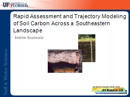
An Example: Study Domain

PLUSES

— DMIP2 Sierra-Nevada Basin in HRAP grid (48×39 grids)

TRIANGLES – East Fork Carson River Basin grid (9×13 grids)DOTS

— SNOTEL & USHCN in-situ sites.

Sierra-Nevada Basins

DMIP2 West - American, Carson

8

MODIS Snow Cover Frac

on

HRAP grid

The snow cover fraction data were derived from Terra-MODIS Level 3 500m Daily Snow Cover Area Data onto a HRAP grid at 4.7625KM resolution. The HRAP grid is treated as cloud cover when the cloud cover fraction is above 50%.

February 2002

9

We perform two runs in parallel. One is without using assimilation (left), and the other is applying the data assimilation (right). We just apply the direct insertion algorithm in our assimilation. The LIS

model

is operating from October 1, 2001 to September 30, 2002.

No DA

With DA

February 2002

February 2002

10

Data Assimilation

(spatial comp.)

Data Assimilation (temporal comp.)

Comparison of snow cover fraction between the MODIS (blue circles), the open loop simulation (black line) and the assimilation simulation (green line).

Comparison of snow water equivalent between the open loop simulation (green), the assimilation simulation (red) and the in-situ measurement (black) averaged over all SNOTEL sites in the study region.

Snow Cover Fraction

Snow Water Equivalent

11

Optimal parameters:

Spatial distribution of in-situ stations consisting of SNOTEL (dots) and USHCN (plus) stations over CONUS. The background colors show the elevation at a 1km resolution as derived from USGS GTOPO30 data.

MODIS FSC retrieval error relative to in-situ

(upper) and NLDAS

(lower) daily mean air temperature for all in-situ sites over CONUS (pluses). The cumulative double exponential distribution function

is

used to construct the nonlinear relationship between the errors and temperature (solid lines).

Quantify MODIS FSC Retrieval Errors

12

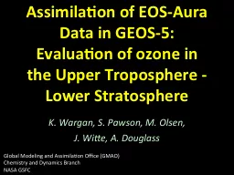
An Example: SMMR SWE assimilation

13

Comparison of the median SWE for pixels including 5 or more stations; ground observations (black dots), SMMR observations (plus), model forecast (dash lines), model forecast with assimilation run-I (dotted lines) and run-II (solid lines) from (a) January to March in 1979 and (b) from July 1986 to June 1987 (zoomed to the winter months from October 1986 to April 1987).

Spatial distribution of all half-degree by half-degree grid cells including 1 to 4 in-situ SWE stations (open squares) and 5 or more in-situ stations (solid squares), with the background colors showing snow classification according to Sturm et al. (1995).

In-situ SWE

SMMR SWE

Model SWE

Feb. 1979

Feb. 1987

14

Difference between model forecast and model forecast with assimilation for monthly averaged total runoff (left column), upward

longwave

radiation (middle column), and upward shortwave radiation (right column) for winter months.

Snow assimilation summary and future plan

Comparison between

open loop and assimilation simulations shows that

both FSC and SWE are improved through the assimilation of MODIS derived FSC.

MODIS FSC retrieval errors can be quantitatively predicted by

temperature, which is a key input for using advanced Kalman

Filter assimilation technique.

Assimilation of SMMR SWE through

Kalman

Filter approach demonstrate a big improvement to model SWE simulation.

We

will apply the derived statistical regression equation to prescribe the error in MODIS snow cover fraction, and further apply into the

EnKF

assimilation.

15