Introduction to Matlab Jefferson Davis - PowerPoint Presentation

Slide1

Introduction to Matlab

Jefferson Davis

Research Analytics

Slide2

Research Analytics

Formerly the Stat/Math Center

A group within the Research Technology (RT) division of University Information Technology Services (UITS)

S

upport, consultation, and administration

for

software in statistics, mathematics, and geographic information systems (GIS)

Slide3

“Research Analytics-y” questions

“Can I use import my data into

Stata

?”

“How do I run

a

Kolmogorov–

Smirnov test

in

Matlab

?”

“My

optimization

takes forever to run. Why?”

“How can I export an ArcGIS attribute table to Excel?”

Slide4

Matlab background

Developed by Cleve

Moler

in the 1970s to give students easier access to numerical

libraries for linear algebra (Matrix Laboratory)

MathWorks

company founded in 1984 for commercial

development

The fundamental

datatype

is the matrix (array)

About 1200 IU network users fall 2013

Slide5

Matlab availability

STC labs

IUAnyware

This is the one we’ll be using

Quarry

“At IU, on

Quarry,

how do I use MATLAB?”

http://

kb.iu.edu

/data/

ayfu.html

Big Red II

"At

IU, on Big Red II, how do I use

MATLAB?”

http

://

kb.iu.edu

/data/

bdns.html

Mason

Get accounts at

itaccounts.iu.edu

Matlab

app

Slide6

Getting to Matlab

on

IUAnyware

We start by going to

iuanyware.iu.edu

Slide7

Getting to

Matlab

on

IUAnyware

If you get this screen,

relax and “Skip to log

on.”

I always get this screen.

Slide8

Getting to

Matlab

on

IUAnyware

Now navigate through

“Analysis & Modeling”

-> “Statistics – Math”

->

Matlab

Slide9

Getting to

Matlab

on

IUAnyware

Now navigate through

“Analysis & Modeling”

-> “Statistics – Math”

->

Matlab

Slide10

Getting to

Matlab

on

IUAnyware

Now navigate through

“Analysis & Modeling”

-> “Statistics – Math”

->

Matlab

Slide11

Taking a look at the interface

Slide12

Arithmeticy stuff in

Matlab

Fortunately, mathematical notation is pretty standardized. Most arithmetic works like you think it should.

2+3

ans

=

5

Matlab

assigns the most recent calculation to

ans

…

a=34*8

a=

272

unless you make

an assignment explicitly

b=a

b=272

pi

ans

=3.1416

Common

constants are available…

i

ans

=0.0000 + 1.0000i

as

are complex numbers.

sin(pi)

ans

=1.2246e-16

Should

we worry this isn’t zero?

eps

ans

= 2.2204e-16

Well it’s smaller than

eps

, we won’t worry.

Slide13

Vectors in Matlab

d=[1

2 3 4 5 6]

d =

1 2 3 4 5 6

d,

e, and f are all equivalent 1 x 6 vectors

e=[1:6]

e =

1 2 3 4 5 6

f=1:6

f

=

1 2 3 4 5 6

g

= 0:2:6

g = 0 2 4 6

sin(g)

ans

= 0 0.9093 -0.7568 -0.2794

Matlab

applies the sine function to each element of g.

g(3)

4

g(1:3)

0 2 4

g'

ans

=

0

2

4

6

Slide14

More Vectors

g

'

ans

=

0

2

4

6

g+g

ans

= 0 4 8 12

g+

g

'

Error using +

Matrix dimensions must agree.

g*g'

ans

= 120

This is matrix multiplication

, or the dot production in this case.

g*g

Error using *

Inner matrix dimensions must agree.

g.*g

ans

=

0 4 16 36 64

Including

the dot tells

Matlab

that you don’t want matrix multiplication but instead want

pointwise

multiplication.

Slide15

Matrices in Matlab

h=[1 2 3; 4 5 6; 7 8 9]

h =

1 2 3

4 5 6

7 8 9

h(2,2)

ans

=

5

Selecting

the entry in the second row second column.

h(2,:)

ans

=

4 5

6

Selecting

the entries in the second row but all columns.

h(:,2:3)

ans

=

2 3

5 6

8 9

Selecting

the entries in the all rows in columns 2-3.

h(3)

ans

=

7

With one

index,

Matlab

counts column-by-column.

h^2

ans

=

30 36 42

66 81 96

102 126 150

This is matrix multiplication.

h.^2

ans

=

1 4 9

16 25 36

49 64 81

With the period we get multiply

the elements of h by themselves

pointwise

.

Slide16

More Matrices

As you would expect,

Matlab

has many functions for creating matrices.

rand(2,3)

ans

=

0.8147 0.1270 0.6324

0.9058 0.9134 0.0975

ones(2)

ans

=

1 1

1 1

This is the same as

ones(2,2)

zeros(1,4)

ans

=

0 0 0 0

This

is the most common way to initialize variables.

a=[1 2;3 4]

a =

1 2

3 4

[a a]

ans

=

1 2 1 2

3 4 3 4

Horizontal concatenation

[a ; a]

ans

=

1 2

3 4

1 2

3 4

Vertical

Slide17

A few useful notes

The help command will display a function’s help text.

The doc command brings up more information

help sin

doc sin

The semi-colon (;) will suppress output

The up arrow key will go back to previous commands

Typing and then using the up arrow key goes back to previous commands that start with that

text

The exclamation point is used for shell commands

!

rm

matlab_crash_dump

.*

The

percent sign is used for comments

%This is a

Matlab

comment

Slide18

Vectorized code

You might from time to time be tempted to create a matrix by defining each element one-by-one in a for loop or something like that. That will work but using

Consider two ways to create a 10,000 x 1 vector

[1, 4, 9, 16,…,10000

2

]

The code on the right is said to be

vectorized

. It’s usually a good idea to try to

vectorize

your code. Just don’t go crazy with it.

tic

a=zeros(1,10000);

for

i

=1:10000

a(

i

)=i^2;

end

toc

tic

a=[1:10000].^2;

toc

Elapsed time is 0.000282 seconds.

Elapsed time is 0.000063 seconds.

Slide19

A note on initializing variables

If you do decide to use a for loop to assign the values, please please try to initialize your variables.

tic

a=zeros(1,10000);

for

i

=1:10000

a(

i

)=i^2;

end

toc

tic

for

i

=1:10000

a(

i

)=i^2;

end

toc

Elapsed time is 0.000282 seconds.

Elapsed time is

0.012829 seconds. Yikes.

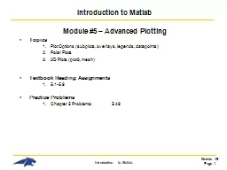
Slide20

Plotting curves in Matlab

It’s pretty straightforward to plot one vector against another in

Matlab

x

=-5:.1:5;

plot(sin(x)

)

Note that both x and sin(x) are vectors of size 1 x 101.

Slide21

Plotting curves in

Matlab

x=-5:.1:5;

plot

(

x,sin

(x

)

, 'g')

Slide22

Plotting curves in

Matlab

figure(2)

plot

(

x,sin

(x),'g')

hold on

plot

(

x,cos

(x),'r-.')

Slide23

Plotting curves in

Matlab

f

igure(3)

subplot(1,2,1)

plot

(

x,sin

(x),'g')

subplot(

1,2,2)

plot

(

x,cos

(x),'r-.'

)

See help plot for more examples

Slide24

Plotting surfaces in

Matlab

Plotting surfaces in

Matlab

is similar to plotting curves.

[x

y

]=

meshgrid

(-5:.1:5,-5:.1:5)

;

z

=x.^2-y.^2

;

mesh

(

x,y,z

)

Here

x,y

, and z are all matrices of size 101 x 101.

Slide25

Plotting surfaces in

Matlab

colormap

(copper)

Slide26

Plotting surfaces in Matlab

set(

gca

,'

CameraPosition

',[45 45 45

])

Slide27

Matlab scripts

Matlab

statements can be saved in a file (m-file) for later use. To save the commands used for

edit saddle

Type the following lines in the

Matlab

editor

[

x y]=

meshgrid

(-5:.1:5,-5:.1:5);

z

=x.^2-y.^2;

mesh

(

x,y,z

)

colormap

(copper

)

and save the file. This will show up as

saddle.m

in your file system. To run the script type

saddle

In the

Matlab

command window.

Slide28

Matlab functions

Writing your own

Matlab

function is similar. To create a function that adds one to a number, type the following in the command window.

edit

addone

Type the following lines in the editor

function y=

addone

(x)

%

Addone

will add one to a matrix

y=x+1;

and save the file. You can run the file like any other

Matlab

function.

addone

(3

)

ans

=

4

In the

Matlab

command window.

Note

both scripts

and

functions are called

m-files.

Slide29

Saving your data

The command save will by default save all of your variables to a file called

matlab.mat

.

Many data formats have support for importing and exporting the data in

Matlab

. This might be native to

Matlab

(e.g.

NetCDF

) or written by users (e.g. FCS)

save(‘

myVars

’,’a’)

Just

save the variable a.

save(‘

myVars.mat’,’a’,’b

’)

Save a and b.

load(‘

myVars.mat

’)

Load the variables in

myVars.mat

load(‘

myVars

’)

This also works

xlswrite

(‘myVars.

xls

’,a)

Write

a to an excel file. (Some issues on Macs)

a=

xlsread

(‘

myVars.xls

’)

Read the excel file and assign to a.

Slide30

Running statistical tests

The Statistical Toolbox has most common stats functions. The code below takes the first column in a matrix of grades and runs a

Kolmogorov-Smirnov

test to test the null hypotheses that the data comes from a normal distribution with mean 75 and standard deviation 10

load

examgrades

;

test1

= grades(:,1);

x

=(test1-75)/10;

[

h p]=

kstest

(x

)

h

=

0

p =

0.561153346365393

hist

(x)

The result h=0 shows

kstest

fails to reject

the null hypothesis at the default 5% level.

Slide31

Matlab mapping functions (GIS)

In the past decade several numerical platforms have started including functions to analyze and display GIS data

In

Matlab

these functions are in the Mapping Toolbox

At IUB we see a lot more on the analysis side rather than on the display side

Even simple examples will have a fair amount of syntax to make

Slide32

GTOPO30 data in Matlab

example

% Extract and display a subset of full resolution data for the state of

%

Massachusetts.

% Read the

stateline

polygon boundary and calculate boundary limits.

Massachusetts =

shaperead

('

usastatehi

', '

UseGeoCoords

', true, ...

'Selector',{@(name)

strcmpi

(

name,'Massachusetts

'), 'Name'})

;

latlim

= [min(

Massachusetts.Lat

(:)) max(

Massachusetts.Lat

(:))];

lonlim

= [min(

Massachusetts.Lon

(:)) max(

Massachusetts.Lon

(:))];

%

Read the gtopo30 data at full resolution.

[

Z,refvec

] = gtopo30('W100N90',1,latlim,lonlim);

%

Display the data grid and

% overlay

the

stateline

boundary.

figure

usamap

('Massachusetts');

geoshow

(Z,

refvec

, '

DisplayType

', 'surface')

geoshow

([

Massachusetts.Lat

],

...

[

Massachusetts.Lon

],'

Color','m

'

)

demcmap

(Z)

Slide33

Thanks for coming

%code to plot a heart shape in MATLAB

%Adapted form http://

www.walkingrandomly.com

/?p=2326

%set up mesh

n=100;

x=

linspace

(-3,3,n);

y=

linspace

(-3,3,n);

z=

linspace

(-3,3,n);

[X,Y,Z]=

ndgrid

(

x,y,z

);

%Compute function at every point in mesh

F=320 * ((-X.^2 .* Z.^3 -9.*Y.^2.*Z.^3/80) ...

+ (X.^2 + 9.* Y.^2/4 + Z.^2-1).^3);

%generate plot

isosurface

(F,0)

view([-67.5 2]);

%Adjust the

colormap

cm=

colormap

('jet');

%Zero out all the green and blue

cm(:,2:3)=0;

colormap

(cm);