Support vector machines When the data is linearly separable, which of the many possible - PowerPoint Presentation

Slide1

Support vector machines

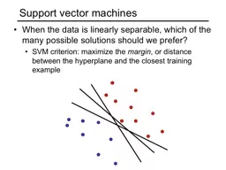
When the data is linearly separable, which of the many possible solutions should we prefer?SVM criterion: maximize the margin, or distance between the hyperplane and the closest training exampleSlide2

Support vector machines

When the data is linearly separable, which of the many possible solutions should we prefer?

SVM criterion: maximize the

margin, or distance between the hyperplane and the closest training example

Margin

Support vectorsSlide3

Finding the maximum margin hyperplane

Define the

margin as the distance between the hyperplane

and the closest point

Distance between point and hyperplane is given by

Assuming the data is linearly separable, we can fix the scale of

and

so that

and

for all other points

Then the margin is

 Slide4

Finding the maximum margin hyperplane

Find separating hyperplane that maximizes the distance to the closest training example

Margin

Support vectors

Positive examples:

Negative examples:

For support vectors,

The margin is

 Slide5

Finding the maximum margin hyperplane

Maximize margin

while correctly classifying all training data:

positive:

negative:

Equivalent problem:

This is a quadratic objective with linear constraints: convex optimization, global optimum can be found using well-studied methods

 Slide6

“Soft margin” formulation

What about non-separable data?

And even for separable data, we may prefer a larger margin with a few constraints violated

SourceSlide7

“Soft margin” formulation

What about non-separable data?

And even for separable data, we may prefer a larger margin with a few constraints violated

SourceSlide8

“Soft margin” formulation

+1

-1

0

Penalize margin violations using

hinge loss

:

Incorrectly classified

Correctly classified

Hinge lossSlide9

“Soft margin” formulation

+1

-1

0

Penalize margin violations using

hinge loss

:

Incorrectly classified

Correctly classified

Hinge loss

Recall hinge loss used by the perceptron update algorithm!Slide10

Penalize margin violations using

hinge loss:

“Soft margin” formulation

Maximize margin –

a.k.a.

regularization

Minimize misclassification lossSlide11

SGD optimization (omitting bias)

Recall:

 Slide12

SGD optimization (omitting bias)

SGD update:

If

:

Otherwise:

S. Shalev-Schwartz et al.,

Pegasos: Primal Estimated sub-

GrAdient

SOlver

for SVM

,

Mathematical Programming

, 2011Slide13

SVM vs. perceptron

SVM loss:

SVM update:

If

:

Otherwise:

Perceptron loss:

Perceptron update:

If

:

Otherwise: do nothing

What are the differences?

 Slide14

Dual SVM formulation

SVM objective:

Directly solving for

using SGD is called the

primal

approach

Instead, SVM optimization can be formulated to learn a classifier in the form

by solving a

dual

optimization problem over

 Slide15

Dual SVM formulation

The dual problem (given without derivation):

Important properties of the dual:

At the optimum,

are nonzero only for support vectors

Feature vectors appear only inside dot products

:

this enables nonlinear SVMs via

kernel functions

 Slide16

Φ

:

x

→

φ

(

x

)

Nonlinear SVMs

General idea: the original input space can always be mapped to some higher-dimensional feature space where the training set is separable

Slide credit: Andrew MooreSlide17

Nonlinear SVMs

The kernel trick: instead of explicitly computing the lifting transformation

,

define a kernel function

To be valid, the kernel function must satisfy

Mercer’s condition

This gives a nonlinear decision boundary in the original feature space:

 Slide18

Non-separable data in 1D:

Apply mapping

:

0

x

0

x

x

2

ExampleSlide19

Kernel example 1: Polynomial

Polynomial kernel with degree and constant

:

What this looks like for

:

Thus, the explicit feature transformation consists of all polynomial combinations of individual dimensions of degree up to

 Slide20

Kernel example 1: PolynomialSlide21

Kernel example 2: Gaussian

Gaussian kernel with bandwith

:

Fun fact: the corresponding mapping

is infinite-dimensional!

||x – x’||

K

(

x, x’

)Slide22

Kernel example 2: Gaussian

Gaussian kernel with bandwith

:

The predictor

is a sum of “bumps” centered on support vectors

SV’s

It’s also called a

Radial Basis Function

(RBF) kernelSlide23

Kernel example 2: Gaussian

Gaussian kernel with bandwith

:

The predictor

is a sum of “bumps” centered on support vectors

How does the value of

affect the behavior of the predictor?

What if

is close to zero?

What if

is very large?

 Slide24

SVM: Pros and cons

Pros

Margin maximization and kernel trick are elegant, amenable to convex optimization and theoretical analysisSVM loss gives very good accuracy in practiceLinear SVMs can scale to large datasets

Kernel SVMs are flexible, can be used with problem-specific kernelsPerfect “off-the-shelf” classifier, many packages are availableCons

Kernel SVM training does not scale to large datasets: memory cost is quadratic and computation cost even worse“Shallow” method: predictor is a “flat” combination of kernel functions of support vectors and test example, no explicit feature representations are learned