Aggregate Demand I: Building the - PowerPoint Presentation

1. Aggregate Demand I: Building the IS-LM ModelChapter 11 of Macroeconomics, 10th edition, by N. Gregory MankiwECO62 Udayan Roy

2. Static Short-Run MacroeconomicsIn this chapter, I will describe the IS-LM theory of static short-run macroeconomics

3. The goods market in the short run

4. Recap of Chapters 3 and 5Long-Run Macroeconomics (Chs. 3, 5) Let’s first look at the real variables (Ch 3) Variables in red font are endogenous. Variables in black font are exogenous.Real variablesGoods MarketsCh. 3Nominal variablesAssets MarketsCh. 5

5. Recap: Equations of Chapter 3Exogenous variables in blackEndogenous variables in red Chapter 3 was about the long run.Now we are discussing the short run. In the short run, the available capital and labor may not be fully utilized.Therefore, the first equation is not applicable in the short run.The other 3 equations continue to apply.

6. Equations from Chapter 3 that are still applicable in the short runExogenous variables in blackEndogenous variables in red Note that there are four unknowns (endogenous variables) and only three equations.We saw in Chapter 1 that to make the theory solvable, the number of unknowns must equal the number of equations.So, we must find ways to make the number of unknowns equal to the number of equations.One approach is the IS-LM theory later in this chapter.We begin with an easier approach called the Keynesian Cross theory.

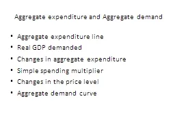
7. The Keynesian CrossThe simplest theory of short-run equilibrium in the goods market

8. The Keynesian Cross TheoryExogenous variables in blackEndogenous variables in red The Keynesian Cross theory assumes that business investment spending is exogenous (that is, inexplicable, like the weather).You may think of this as assuming that the real interest rate, r, is exogenous and that therefore is also exogenous.The equation is now unnecessary. 

9. The Keynesian Cross TheoryExogenous variables in blackEndogenous variables in red Now, you have two endogenous variables, output (Y) and consumption spending (C), in two equations.So, the Keynesian Cross theory can be solved!See the next slide.

10. Keynesian Cross Theory Note that every variable on the right hand-side of the last equation is exogenous. So, this equation is a solution equation. It tells us everything we can say about Y in the Keynesian Cross model.Our first equation makes the supply of goods and services (Y) equal to the demand for goods and services (C + I + G). The textbook refers to the demand for goods and services as planned expenditure: PE = C + I + G. So, the goods market equilibrium equation can also be written as Y = PE.

11. Short-Run GDP: predictionsPredictions GridYCo+T−I+G+Important: Note that there is absolutely no reason why this short-run equilibrium GDP has to be equal to the long-run equilibrium GDP () that we studied in Chapter 3.In other words, the Keynesian Cross model is able to explain why recessions (Y < ) and booms (Y > ) happen. Recall from Ch. 3 that:The first row of the predictions grid lists endogenous variables (unknowns)In this case, Y is the only endogenous variableThe first column lists exogenous variables (knowns)In this case, C0, T, I and G are the exogenous variablesEach cell shows the kind of effect that the corresponding exogenous variable has on the corresponding endogenous variableQ: Can you look at the solution equation for short-run output and see why it algebraically implies the predictions in the predictions grid?

12. The Keynesian Cross EquationLet’s rewrite the Keynesian Cross solution for short-run GDP:

13. The Spending MultiplierNote that if Co + I + G increases by $1.00, then Y increases by $1/(1 – Cy).We saw in Ch. 3 that Cy is the marginal propensity to consume or MPC.So, 1/(1 – Cy) may be written as 1/(1 – MPC).This is called the Keynesian Cross spending multiplier. 

14. The Spending MultiplierAs the marginal propensity to consume is a positive fraction (0 < MPC < 1), 1 – MPC is also a positive fraction. Therefore, 1/(1 – MPC) > 1.So, for every $1.00 increase in Co + I + G, Y increases by more than $1.00!Why??? 

15. The Spending MultiplierSuppose the government spends an additional $1 billion to build a new highwayThis immediately increases national income by $1 billion, because the money spent by the government can’t disappear into thin air; it must end up in people’s pocketsThose who earn this additional income will spend a fraction of it on additional consumption spending (on, say, food)If the MPC is 0.8, this additional spending will be 0.8 × $1 billion or $800 million

16. The Spending MultiplierSo you see that although the government got the ball rolling by spending $1 billion, and in a mere two steps national income has already increased by $1.8 billionThis explains why the spending multiplier is greater than one… and the process will continue!Those who produced the additional food bought by those who made the highway will earn $800 millionThey will spend 0.8 × $800 million or $640 million on additional consumption (of, say, clothes), and so on and on …

17. The Spending MultiplierRecall that the spending multiplier is 1/(1 – MPC).Example: If MPC = 0.2, the spending multiplier = 1/(1 – 0.2) = 1.25.Therefore, if a government increases (respectively, decreases) spending by $3 billion, real GDP will increase (respectively, decrease) by $3.75 billionExample: If MPC = 0.8, the spending multiplier = 1/(1 – 0.8) = 5.Therefore, if a government increases (respectively, decreases) spending by $3 billion, real GDP will increase (respectively, decrease) by $15 billion

18. The Spending MultiplierRecall that the spending multiplier is 1/(1 – MPC).Example: If MPC = 0.2, the spending multiplier = 1/(1 – 0.2) = 1.25.Therefore, if a government increases (respectively, decreases) spending by $3 billion, real GDP will increase (respectively, decrease) by $3.75 billionExample: If MPC = 0.8, the spending multiplier = 1/(1 – 0.8) = 5.Therefore, if a government increases (respectively, decreases) spending by $3 billion, real GDP will increase (respectively, decrease) by $15 billionThe Keynesian Cross theory assumes that the economy is in a recession and, therefore, has unemployed resources.

19. The Spending MultiplierRecall that the spending multiplier is 1/(1 – MPC).Example: If MPC = 0.2, the spending multiplier = 1/(1 – 0.2) = 1.25.Therefore, if a government increases (respectively, decreases) spending by $3 billion, real GDP will increase (respectively, decrease) by $3.75 billionExample: If MPC = 0.8, the spending multiplier = 1/(1 – 0.8) = 5.Therefore, if a government increases (respectively, decreases) spending by $3 billion, real GDP will increase (respectively, decrease) by $15 billionThe bigger MPC is, the bigger the spending multiplier will be. (Why??)

20. The Spending MultiplierRecall that the spending multiplier is 1/(1 – MPC).Example: If MPC = 0.2, the spending multiplier = 1/(1 – 0.2) = 1.25.Therefore, if a government increases (respectively, decreases) spending by $3 billion, real GDP will increase (respectively, decrease) by $3.75 billionExample: If MPC = 0.8, the spending multiplier = 1/(1 – 0.8) = 5.Therefore, if a government increases (respectively, decreases) spending by $3 billion, real GDP will increase (respectively, decrease) by $15 billionSo, being big savers (low MPC) weakens the effect of government spending on real GDP.

21. The Tax-Cut MultiplierNote that if net tax revenue (T) decreases by $1.00, then Y increases by $Cy/(1 – Cy).As Cy is the marginal propensity to consume, Cy /(1 – Cy) may be written as MPC/(1 – MPC).This is the Keynesian Cross tax-cut multiplier. 

22. The Tax-Cut MultiplierAs the marginal propensity to consume is a positive fraction (0 < MPC < 1), MPC/(1 – MPC) < 1/(1 – MPC) Tax-cut multiplier < spending multiplierThat is, a $1.00 tax cut provides a smaller boost to the economy than a $1.00 increase in government spending. (Why??) At this point, you should be able to do problems 1 and 2 (b) – (e) on page 330 of the textbook. Please try.

23. The Tax-Cut MultiplierWhy is it that a $1.00 tax cut provides a smaller boost to the economy than a $1.00 increase in government spending?A $1 increase in government spending is guaranteed to increase national income by $1 right away (because the money spent by the government can’t disappear into thin air; it must end up in people’s pockets).But a fraction 1 – MPC of a $1 tax cut will be saved.So, the tax cut will not have as big an effect as direct government spending

24. The Tax-Cut MultiplierIf MPC = 0.2, the tax-cut multiplier = 0.2/(1 – 0.2) = 0.25 < 1.Therefore, if the government cuts (respectively, raises) taxes by $3 billion, real GDP will increase (respectively, decrease) by $0.75 billionIf MPC = 0.8, the tax-cut multiplier = 0.8/(1 – 0.8) = 4 > 1. Therefore, if the government cuts (respectively, raises) taxes by $3 billion, real GDP will increase (respectively, decrease) by $12 billionSo, being big savers (low MPC) weakens the effect of taxes on real GDP. 

25. The Balanced-Budget MultiplierRecall from Ch. 3 that the government’s saving is T – G.A government that wishes to keep its budget balanced will need to match any change in government purchases (G) with an equal change in it net tax revenue (T). 

26. The Balanced-Budget MultiplierA one dollar increase in G will increase Y by dollarsA one dollar increase in T will decrease Y by dollarsSo the overall effect of this balanced-budget increase in both G and T is that Y will increase by dollar.That is, the Keynesian Cross balanced-budget multiplier is 1. 

27. The MultipliersMPC(a)Spending Multiplier(b)Tax-Cut Multiplier(c)Balanced-Budget Multiplier(b) – (c)0.11.110.111.000.21.250.251.000.52.001.001.000.85.004.001.000.910.009.001.00Note again that if people save more (lower MPC), the spending and tax-cut multipliers are smaller.Therefore, in short-run macroeconomics, low-saving weakens the effectiveness of government fiscal (or taxing and spending) policy.

28. Fiscal PolicyThe practice of changing the levels of government spending (G) and/or taxes (T) in order to affect the macroeconomic outcome is called fiscal policySpending more (G↑) and/or cutting taxes (T↓) is called expansionary fiscal policy (or “stimulus”)This decreases government saving (T – G↓)Spending less (G↓) and/or raising taxes (T↑) is called contractionary fiscal policy (or “austerity” or “belt tightening”)This increases government saving (T – G↑)

29. Tax Cuts: JFKKennedy cut personal and corporate income taxes in 1964An economic boom followed. GDP grew 5.3% in 1964 and 6.0 in 1965. Unemployment fell from 5.7% in 1963 to 5.2% in 1964 to 4.5% in 1965.However, it is not easy to prove that the tax cuts caused the boomEven when they agree that the tax cuts caused the boom, economists can’t agree on the reason

30. Tax Cuts: JFKKeynesians argued that the tax cuts boosted demand, which led to higher production and falling unemploymentSupply-siders argued that demand had nothing to do with it. The tax cuts gave people the incentive to work harder. So, L increased. Therefore, Y = F(K, L) also increased.Personally, I feel this argument doesn’t explain why the unemployment rate fell

31. Tax Cuts: GWBBush cut taxes in 2001 and 2003After the second tax cut, a weak recovery from the 2001 recession turned into a strong recoveryGDP grew 4.4% in 2004Unemployment fell from its peak of 6.3% in June 2003 to 5.4% in December 2004In justifying his tax cut, Bush used the Keynesian explanation: “When people have more money, they can spend it on goods and services. … when they demand an additional good or service, somebody will produce the good or service.”

32. Spending Stimulus: Barack ObamaWhen President Obama took office in January 2009, the economy had suffered the worst collapse since the Great DepressionObama helped enact an $800 billion (5% of annual GDP) stimulus to be spent over a two-year periodAbout 40% was tax cuts, and 60% was additional government spendingWhite House economists had estimated the spending multiplier to be 1.57 and the tax-cut multiplier to be 0.99

33. Spending Stimulus: Barack ObamaMuch of the new spending was on infrastructure projectsThese projects were fine for the long run, but took a long time to be implemented, and were therefore not ideal as a short-run boostObama publicly justified his stimulus bill using Keynesian demand-side reasoning

34. Big-Picture ComparisonLong-Run Macroeconomics Short-Run Macroeconomics (Keynesian Cross) Variables in red font are endogenous. Variables in black font are exogenous.Real variablesGoods MarketsCh. 3Nominal variablesAssets MarketsCh. 5

35. The Keynesian Cross Theory: WarningsThe theory assumes that the economy is in a recession and has unutilized labor and capital. If the economy has already reached full employment, any efforts to further increase demand will cause problems.The theory I have discussed assumes a closed economy. In an open economy, policies designed to increase demand may lead to higher demand, but for imported goods.Interest rates and inflation rates play no role in this theory.

36. The is-lm theory of static short-run macroeconomics

37. Recap of Chapters 3 and 5Long-Run Macroeconomics (Chs. 3, 5) IS-LM Theory Variables in red font are endogenous. Variables in black font are exogenous.Real variablesGoods MarketsCh. 3Nominal variablesAssets MarketsCh. 51. The output equation makes no sense in short-run macroeconomics because K and L may not be fully employed all the time.2. Prices are “sticky” or “rigid” in short-run macroeconomics. So, P becomes exogenous.

38. Recap of Chapters 3 and 5Long-Run Macroeconomics (Chs. 3, 5) IS-LM Theory Variables in red font are endogenous. Variables in black font are exogenous.Real variablesGoods MarketsCh. 3Nominal variablesAssets MarketsCh. 53. π is the rate of inflation. So it is the growth rate of the price level, P. As P is exogenous, π is exogenous too. So the long-run inflation equation has no endogenous variable in it. Therefore, it is of no use in understanding our endogenous variables. So, this equation can go.

39. Recap of Chapters 3 and 5Long-Run Macroeconomics (Chs. 3, 5) IS-LM Theory Variables in red font are endogenous. Variables in black font are exogenous.Real variablesGoods MarketsCh. 3Nominal variablesAssets MarketsCh. 54. In Ch. 5, this equation for the ex ante real interest rate (r) was originally i = r + Eπ, where Eπ was defined as expected inflation. In the IS-LM theory we will return to that equation. Moreover, it is assumed that expected inflation (Eπ) is exogenous.

40. Recap of Chapters 3 and 5Long-Run Macroeconomics (Chs. 3, 5) IS-LM Theory Equations Variables in red font are endogenous. Variables in black font are exogenous.Real variablesGoods MarketsCh. 3Nominal variablesAssets MarketsCh. 5Now we have the final set of equations for the IS-LM theory of short-run macroeconomics.Note that the IS-LM theory has 5 endogenous variables (unknowns) and 5 equations. So, chances are that the theory might work!

41. The IS-LM TheoryGoods market equilibrium conditionsAssets market equilibrium conditions LMISYr1. The goods market equilibrium equations will give us the IS curve, an inverse relation between the real interest rate (r) and real output (Y).2. The assets market equilibrium equations will give us the LM curve, a direct relation between the real interest rate (r) and real output (Y).3. The intersection of the IS and LM curves will give us the short-run macroeconomic outcomes for r and Y.4. From Y we’ll know C. And from r we’ll know both I and i. That would help us make testable predictions about all of our five endogenous variables.

42. The IS CurveA slightly more complex theory of short-run equilibrium in the goods market

43. The IS CurveGoods market is in equilibrium when … Endogenous variables in red 

44. Deriving the IS Curve: algebraK.C. Spending multiplierK.C. Tax-cut multiplierIS Interest rate effect

45. Comparing the Equations of the Keynesian Cross and the IS CurveKeynesian CrossIS CurveK.C. Spending multiplierK.C. Tax-cut multiplierIS Interest rate effectK.C. Spending multiplierK.C. Tax-cut multiplierThis is the only difference

46. The IS CurveK.C. Spending multiplierK.C. Tax-cut multiplierIS Interest rate effectY2Y1rY r1ISr2ΔYΔrAny change in the real interest rate will cause an opposite change in real total GDP by a multiple determined by the size of the interest rate effect.This is why the IS curve is negatively sloped.

47. The IS Curve: effect of fiscal policyK.C. Spending multiplierK.C. Tax-cut multiplierIS Interest rate effectY2Y1rY r1IS1IS2YAny increase in Co + Io + G causes the IS curve to shift right by the amount of the increase magnified by the Keynesian Cross spending multiplierNote that if the real interest rate is unchanged, the Keynesian Cross model is the same as the IS curve model.

48. The IS Curve: effect of fiscal policyK.C. Spending multiplierK.C. Tax-cut multiplierIS Interest rate effectY2Y1rY r1IS1IS2YAny decrease in taxes (T) causes the IS curve to shift right by the amount of the tax cut magnified by the Keynesian Cross tax-cut multiplier

49. The IS Curve: effect of fiscal policyK.C. Spending multiplierK.C. Tax-cut multiplierIS Interest rate effectY2Y1rY r1IS1IS2YIf both G and T increase by, say, five dollars, the IS curve will shift right by five dollars. (Recall that the Keynesian Cross balanced-budget multiplier is exactly 1.

50. The IS Curve: shiftsTo sum up the previous two slides:The IS curve shifts right if there is:an increase in Co + Io + G, ora decrease in T , ora balanced-budget increase in both G and T.

51. The money market in the short run: the LM CurveThe “liquidity preference” theory of short-run equilibrium in the money market

52. Copy of earlier slide: The IS-LM TheoryGoods market equilibrium conditionsAssets market equilibrium conditions LMISYr1. The goods market equilibrium equations will give us the IS curve, an inverse relation between the real interest rate (r) and real output (Y).2. The assets market equilibrium equations will give us the LM curve, a direct relation between the real interest rate (r) and real output (Y).3. The intersection of the IS and LM curves will give us the short-run macroeconomic outcomes for r and Y.4. From Y we’ll know C. And from r we’ll know both I and i. That would help us make testable predictions about all of our five endogenous variables.

53. Money Supply = Money DemandIn Chapter 5, we used the specific form to indicate that our desire for liquidity is inversely related to the nominal interest rate, i.So, the above equation becomes .Therefore, we get:  

54. Money Demand = Money SupplyNow, recall from Chapter 5 that the ex ante real interest rate (r) is the nominal interest rate (i) minus the expected inflation rate (Eπ): r = i – EπTherefore, r + Eπ = iSo, the money market equilibrium equation becomes  At this point, you should be able to do problem 5 on page 330 of the textbook. Please try it.

55. Real Money BalancesThe term M/P is called real money balances.One may think of M/P as the purchasing power of the nation’s quantity of money or money supply.Example: If you have $10 and the price of a cup of coffee is $4, then your purchasing power is 10/4 = 2.5 cups of coffee 

56. The LM EquationTraditionally, this equation is called the LM equation 

57. Money Demand = Money SupplyAssumption: As always, the money supply (M), which is controlled by the central bank, is exogenousAssumption: Unlike the long-run analysis of Chapter 5, expected inflation (Eπ) is exogenous in the short run.Assumption: Unlike the long-run analysis of Chapter 5, the overall price level (P) is exogenous in the short run.So, Y and r are the only endogenous variables (unknowns) in the LM equation 

58. Money Demand = Money SupplyLM equation:So, if the real interest rate (r) increases, then real GDP (Y) must increase too, in order to keep money demand equal to money supplyThis result gives us a new curve, the LM curve 

59. The LM Curve: algebra to graphThe LM curve shows all combinations of the real interest rate (r) and real output (Y) for which the money market is in equilibriumNote that the LM curve is upward risingrYY1r1r2Y2LM 

60. The LM Curve: algebra to graphThe LM curve shifts (down) right if:Real money balances (M/P) or expected inflation (Eπ) increases, orFear of non-liquid assets (Lo) decreasesMoreover, if Eπ increases, the LM curve shifts down by the exact same amount!!rYr2Y0LM1LM2r1 

61. Bonus Topic: Deducing Inflation ExpectationsRecall from Chapter 5 that the ex ante real interest rate (r) is the nominal interest rate (i) minus the expected inflation rate (Eπ): r = i – EπSo, Eπ = i – r.Luckily, we can easily get data on both the nominal interest rate (i) and the real interest rate (r).So, we can deduce the inflation that people are expecting, on average, by calculating Eπ = i – r.This is called the breakeven expected inflation rate.

62. Bonus Topic: Deducing Inflation ExpectationsHere’s one measure of the nominal interest rate (i): 10-Year Treasury Constant Maturity Securities (DGS10)Here’s one measure of the real interest rate (r): and 10-Year Treasury Inflation-Indexed Constant Maturity Securities (DFII10)As Eπ = i – r, by subtracting the real interest rate from the nominal interest rate, we get a measure of expected inflation: 10-Year Breakeven Inflation Rate (T10YIE)

63. Bonus Topic: Deducing Inflation Expectations

64. Bonus Topic: Deducing Inflation ExpectationsNominalRealExpected Inflation = Nominal - Real

65. Bonus Topic: Deducing Inflation ExpectationsThis is another measure of expected inflation: https://fred.stlouisfed.org/series/T5YIFR. It is a measure of expected inflation (on average) over the five-year period that begins five years from a specified day.

66. The LM Curve: algebra to graphNote that the LM equation can be written as:This implies: rYr2Y0LM1LM2r1 

67. The LM Curve: algebra to graphAs L0, P, M, and Eπ are exogenous, if Eπ increases, then L0, P, and M will be unaffected.Moreover, if Y remains unchanged at, say, Y0, then, according to the LM equation, r must decrease by the same amount as the increase in Eπ. rYr2Y0LM1LM2r1 

68. The LM Curve: algebra to graphWe just saw that, if Y remains unchanged at, say, Y0, then, according to the LM equation, r must decrease by the same amount as the increase in Eπ.So, if expected inflation increases by some amount, the LM curve must shift down by the same amountThis will be useful in Ch. 12rYr2Y0LM1LM2r1 

69. Short-run equilibrium in the is-lm modelBoth the goods market and the money market need to be in equilibrium

70. The IS-LM theory of short-run macroeconomic equilibriumThe short-run macroeconomic equilibrium is the combination of r and Y that simultaneously satisfies the equilibrium conditions in both the goods and money marketsReal output (Y) and real interest rate (r) must satisfy:Y = C(Y – T) + I(r) + G andM = L(r + Eπ)PYY rISLMEquilibriuminterestrateEquilibriumlevel ofincome

71. The IS-LM theory of short-run macroeconomic equilibriumNote that the short-run IS-LM equilibrium GDP does not have to be equal to the long-run equilibrium GDP (; see Ch. 3)Thus, like the Keynesian Cross model, the IS-LM model can explain recessions and booms.But, while the Keynesian Cross model could determine only equilibrium output, the IS-LM model determines the equilibrium real interest rate as well. Y rISLMEquilibriuminterestrateEquilibriumlevel ofincome 

72. The IS-LM Model: summaryShort-run equilibrium in the goods market is represented by a downward-sloping IS curve linking Y and r.Short-run equilibrium in the money market is represented by an upward-sloping LM curve linking Y and r.The intersection of the IS and LM curves determine the short-run equilibrium values of Y and r.The IS curve shifts right if there is:an increase in Co + Io + G, ora decrease in T.The LM curve shifts right if:M/P or Eπ increases, orLo decreasesY rISLM

73. Big-Picture ComparisonLong-Run Macroeconomics (Chs. 3, 5) Short-Run Macroeconomics (IS-LM) Variables in red font are endogenous. Variables in black font are exogenous.

74. Preview of Chapter 12In Chapter 12, we willuse the IS-LM model to analyze the impact of policies and shocks.use the IS-LM model to explain the Great Depression.