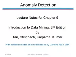
PPT-Data Mining: Data Lecture Notes for Chapter 2

Author : anastasia | Published Date : 2023-07-28

Introduction to Data Mining 2 nd Edition by Tan Steinbach Kumar Outline Attributes and Objects Types of Data Data Quality Similarity and Distance Data Preprocessing

Presentation Embed Code

Download Presentation

Download Presentation The PPT/PDF document "Data Mining: Data Lecture Notes for Chap..." is the property of its rightful owner. Permission is granted to download and print the materials on this website for personal, non-commercial use only, and to display it on your personal computer provided you do not modify the materials and that you retain all copyright notices contained in the materials. By downloading content from our website, you accept the terms of this agreement.

Data Mining: Data Lecture Notes for Chapter 2: Transcript

Introduction to Data Mining 2 nd Edition by Tan Steinbach Kumar Outline Attributes and Objects Types of Data Data Quality Similarity and Distance Data Preprocessing What is Data Collection of . Chapter 1. Kirk Scott. Iris . virginica. 2. Iris . versicolor. 3. Iris . setosa. 4. 1.1 Data Mining and Machine Learning. 5. Definition of Data Mining. The process of discovering patterns in data.. (The patterns discovered must be meaningful in that they lead to some advantage, usually an economic one.). Chapter 1. Kirk Scott. Iris . virginica. 2. Iris . versicolor. 3. Iris . setosa. 4. 1.1 Data Mining and Machine Learning. 5. Definition of Data Mining. The process of discovering patterns in data.. (The patterns discovered must be meaningful in that they lead to some advantage, usually an economic one.). Emre Eftelioglu. 1. What is Knowledge Discovery in Databases?. Data mining is actually one step of a larger process known as . knowledge discovery in databases. (KDD).. The KDD process model consists of six phases. AD103 - Friday, 3pm-4pm. Ben . Langhinrichs. President of Genii Software. Introduction. Ben Langhinrichs, Genii Software. When I am not developing software, I write children’s books and draw pictures.. Iris . virginica. 2. Iris . versicolor. 3. Iris . setosa. 4. 1.1 Data Mining and Machine Learning. 5. Definition of Data Mining. The process of discovering patterns in data.. (The patterns discovered must be meaningful in that they lead to some advantage, usually an economic one.). Iris . virginica. 2. Iris . versicolor. 3. Iris . setosa. 4. 1.1 Data Mining and Machine Learning. 5. Definition of Data Mining. The process of discovering patterns in data.. (The patterns discovered must be meaningful in that they lead to some advantage, usually an economic one.). in Robotics Engineering. Blink . Sakulkueakulsuk. D. . Wilking. , and T. . Rofer. , . Realtime. Object Recognition . Using Decision . Tree . Learning, 2005. . http. ://. www.informatik.uni-bremen.de/kogrob/papers/rc05-objectrecognition.pd. 9. Introduction to Data Mining, . 2. nd. Edition. by. Tan. , Steinbach, Karpatne, . Kumar. With additional slides and modifications by Carolina Ruiz, WPI. 11/20/2018. Introduction to Data Mining, 2nd Edition. Professor Tom . Fomby. Director. Richard B. Johnson Center for Economic Studies. Department of Economics. SMU. May 23, 2013. Big Data:. Many Observations on Many Variables . Data File. OBS No.. Target Var.. Instructor: . Yizhou. Sun. yzsun@ccs.neu.edu. January 6, 2013. Chapter 1. : Introduction. Course Information. Class . homepage: . http://. www.ccs.neu.edu/home/yzsun/classes/2013Spring_CS6220/index.htm. Core Methods in Educational Data Mining EDUC 691 Spring 2019 Assignment BA4 Questions? Comments? Concerns? Association Rule Mining Today’s Class The Land of Inconsistent Terminology Association Rule Mining Introduction to Data Mining, 2. nd. Edition. by. Tan, Steinbach, Karpatne, Kumar. 4/12/2021. Introduction to Data Mining, 2nd Edition Tan, Steinbach, . Karpatne. , Kumar. 1. Anomaly/Outlier Detection. Credit: Gaby . Matalon. What is Data Mining?. The. . process . of analyzing data from different perspectives and summarizing it into useful information. It . uncovers patterns . in a large set of data. Bamshad Mobasher. DePaul University. 2. From Data to Wisdom. Data. The raw material of information. Information. Data organized and presented by someone. Knowledge. Information read, heard or seen and understood and integrated.

Download Document

Here is the link to download the presentation.
"Data Mining: Data Lecture Notes for Chapter 2"The content belongs to its owner. You may download and print it for personal use, without modification, and keep all copyright notices. By downloading, you agree to these terms.