
They replace the value of an image pixel with a combination of its neighbors Basic operations in images Shift Invariant Linear Thanks to David Jacobs for the use of some slides Consider 1D images ID: 533283
Download Presentation The PPT/PDF document "Correlation and Convolution" is the property of its rightful owner. Permission is granted to download and print the materials on this web site for personal, non-commercial use only, and to display it on your personal computer provided you do not modify the materials and that you retain all copyright notices contained in the materials. By downloading content from our website, you accept the terms of this agreement.


Slide1
Correlation and ConvolutionThey replace the value of an image pixel with a combination of its neighbors
Basic operations in images
Shift Invariant
Linear
Thanks to David Jacobs for the use of some slidesSlide2
Consider 1D images
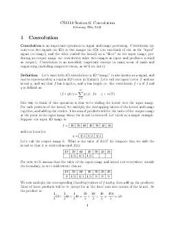
I = [ 5 4 2 3 7 4 6 5 3 6 ]
so I(1)=5, I(2)=4, and so on.
C
onsider
a
simple averaging
operation, in which we replace every pixel in a 1D image by the average
of that
pixel and its two
neighbors, and we produce a new image J. So, J(3) = (I(2)+I(3)+I(4))/3 =(4+2+3)/3=3.
How to deal with boundaries? What is the left neighbor of 5?
(a) [.. 0 0 0
5 4 2 3 7 4 6 5 3 6
0 0 ..] padded with
zeros
[.. 5 5 5
5 4 2 3 7 4 6 5 3 6
6 6 ..] padded with 1
st
and last value
[.. 5 3 6
5 4 2 3 7 4 6 5 3 6
5 4 ..] image repeated cyclicSlide3
Correlation: a sliding operation in a windowSlide4
Continue with next pixelSlide5
Filters
The numbers we multiply with, i.e. (1/3,1/3,1/3) form a filter. This filter is 3 pixels wide.
We could build a filter for averaging that includes a pixel, its neighbors and their neighbors. This filter would be (1/5,1/5,1/5,1/5,1/5) and would be 5 pixels wide. These are “box” filters.
We place the filter on the image, multiply the contents of every cell with the pixel below and add up the results.
For this filter, the new image would be
J(1) = (I(-1)/5 + I(0)/5 + I(1)/5 + I(2)/5 + I(3)/5) = 1+1+1+4/5 + 2/5 = 4 1/5.Slide6
Mathematical DefinitionSuppose F is a correlation filter. It will be convenient
notationally
to suppose that F has an odd number of elements, so we can suppose that as it shifts, its center is right on top of an element of I. So we say that F has 2N+1 elements, and that these are indexed from -N to N, so that the center element of F is F(0). Slide7
Examples in 2DSlide8Slide9
Making filters from continuous functionsSlide10
We would need to evaluate the Gaussian G at points (…,-3,-2,-1,0,1,2,3,..).
Luckily G(x) tends to zero pretty quickly as x gets larger.Slide11
Taking derivatives with filtersSlide12
Matching with correlationMatching the filter with part of the image – their difference depends on 3 terms: the higher the correlation the better the matchSlide13
Weaknesses of correlation
Suppose we correlate the filter:
Notice that we get a high result (85) when we center the filter on the sixth pixel, because (3,7,5) matches very well with (3,8,4). But, the highest correlation occurs at the 13th pixel, where the filter is matched to (7,7,7). Even though this is not as similar to (3,7,5), its magnitude is greater. Slide14
MatchingSlide15
Normalized correlation
When we perform normalized correlation between (3,7,5) and the image I we get image J:
Now, the region of the image that best matches the filter is (3,8,4). However, we also get a very good match between (3,7,5) and end of the image, which, when we replicate the last pixel at the boundary, is (1,2,2). These are actually quite similar, up to a scale factor. Keep in mind that normalized correlation would say that (3,6,6) and (1,2,2) match perfectly. Normalized correlation is particularly useful when some effect, such as changes in lighting or the camera response, might scale the intensities in the image by an unknown factor. Slide16
Correlation as an inner productSlide17
2D correlationSlide18
ExamplesSlide19
ExamplesSlide20
ExampleSlide21
Separable filtersSlide22
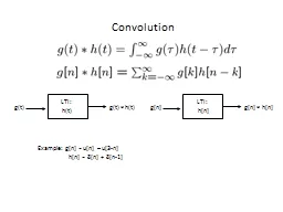
ConvolutionSlide23
ExampleSlide24
Correlation - ConvolutionConvolution is associative (F*G)*H=F*(G*H)
This is very convenient in filtering. If D is a derivative filter and G a smoothing filter then if I is the image: D*(G*I)= (D*G)*I
Correlation is not associative – it is mostly used in matching, where we do not need to combine different filters.Slide25
Dealing with Noise(other presentation)Slide26
Noise
Image
processing is
useful
for noise
reduction...
Common
types of
noise:
Salt
and pepper noise
: contains random occurrences of black and white
pixels
Impulse
noise:
contains random occurrences of white
pixels
Gaussian
noise
: variations in intensity drawn from a Gaussian normal distributionSlide27
Additive noise
I = S + N. Noise doesn’t depend on signal.
We’ll consider:
We often assume the noise is additiveSlide28
Practical noise reduction
How can we “smooth” away noise in a single image
?
0
0
0
0
0
0
0
0
0
0
0
0
0
0
0
0
0
0
0
0
0
0
0
100
130
110
120
110
0
0
0
0
0
110
90
100
90
100
0
0
0
0
0
130
100
90
130
110
0
0
0
0
0
120
100
130
110
120
0
0
0
0
0
90
110
80
120
100
0
0
0
0
0
0
0
0
0
0
0
0
0
0
0
0
0
0
0
0
0
0
0
0
0
0
0
0
0
0
0
0Slide29
Mean filtering
0
0
0
0
0
0
0
0
0
0
0
0
0
0
0
0
0
0
0
0
0
0
0
90
90
90
90
90
0
0
0
0
0
90
90
90
90
90
0
0
0
0
0
90
90
90
90
90
0
0
0
0
0
90
0
90
90
90
0
0
0
0
0
90
90
90
90
90
0
0
0
0
0
0
0
0
0
0
0
0
0
0
90
0
0
0
00000000000000Slide30Slide31
Mean filtering
0
0
0
0
0
0
0
0
0
0
0
0
0
0
0
0
0
0
0
0
0
0
0
90
90
90
90
90
0
0
0
0
0
90
90
90
90
90
0
0
0
0
0
90
90
90
90
90
0
0
0
0
0
90
0
90
90
90
0
0
0
0
0
90
90
90
90
90
0
0
0
0
0
0
0
0
0
0
0
0
0
0
90
0
0
0
00000000000000
0
10203030302010020406060604020030609090906030030508080906030030508080906030020305050604020102030303030201010101000000Slide32
Effect of mean filtersSlide33
Cross-correlation filtering
Let’s write this down as an equation. Assume the averaging window is (2k+1)x(2k+1):
We
can generalize this idea by allowing different weights for different neighboring pixels:
This
is called a
cross-correlation
operation and written:
H
is called the “filter,” “kernel,” or “mask.”
The above allows negative filter indices. When you implement need to use: H[
u+k,v+k
] instead of H[
u,v
]Slide34
Mean kernelWhat’s the kernel for a 3x3 mean filter?
0
0
0
0
0
0
0
0
0
0
0
0
0
0
0
0
0
0
0
0
0
0
0
90
90
90
90
90
0
0
0
0
0
90
90
90
90
90
0
0
0
0
0
90
90
90
90
90
0
0
0
0
0
90
0
90
90
90
0
0
0
0
0
90
90
90
90
90
0
0
0
0
0
0
0
0
0
0
0
0
0
0
90
0
0
0
00000000000000Slide35
Gaussian Filtering
A Gaussian kernel gives less weight to pixels further from the center of the window
This
kernel is an approximation
of
a Gaussian function:
0
0
0
0
0
0
0
0
0
0
0
0
0
0
0
0
0
0
0
0
0
0
0
90
90
90
90
90
0
0
0
0
0
90
90
90
90
90
0
0
0
0
0
90
90
90
90
90
0
0
0
0
0
90
0
90
90
90
0
0
0
0
0
90
90
90
90
90
0
0
0
0
0
0
0
0
0
0
0
0
0
09000000000000000000
1
21242121Slide36
Gaussian Averaging
Rotationally
symmetric.
Weights nearby pixels more than distant ones.
This makes sense as
probabilistic
inference.
A Gaussian gives a good model of a fuzzy blobSlide37
An Isotropic Gaussian
The picture shows a smoothing kernel proportional to
(which is a reasonable model of a circularly symmetric fuzzy blob)Slide38
Mean vs. Gaussian filteringSlide39
Efficient Implementation
Both, the BOX filter and the Gaussian filter are separable:
First convolve each row with a 1D filter
Then convolve each column with a 1D filter.Slide40
Convolution
A
convolution
operation is a cross-correlation where the filter is flipped both horizontally and vertically before being applied to the image:
It
is written:
Suppose H is a Gaussian or mean kernel. How does convolution differ from cross-correlation?Slide41
Linear Shift-InvarianceA tranform T{} is
Linear if:
T(a g(x,y)+b h(x,y)) = a T{g(x,y)} + b T(h(x,y))
Shift invariant if:
Given T(i(x,y)) = o(x,y)
T{i(x-x0, y- y0)} = o(x-x0, y-y0)Slide42
Median filters
A
Median Filter
operates over a window by selecting the median intensity in the window.
What advantage does a median filter have over a mean filter?
Is a median filter a kind of convolution?
Median filter is non linearSlide43
Comparison: salt and pepper noiseSlide44
Comparison: Gaussian noiseSlide45
Fourier Series
Analytic geometry gives a coordinate
system for describing geometric objects
.
(
x,y
) = x(1,0) + y (0,1)
(1,0) and (0,1) form
an orthonormal basis for the plane. That means they are
orthogonal – their inner product <(
1,0), (0,1)> = 0, and of unit magnitude.
Fourier
Series
gives a
coordinate system for functions.Slide46
Why is an orthonormal basis a good representation? Projection.
To find the x coordinate, we take <(
x,y
), (1,0
)>.
Pythagorean
theorem
. Slide47
What is the inner product for functions
With discrete vectors, to compute the inner product we multiply together the values of matching coordinates, and then add up the results. We do the same thing with continuous functions; we multiply them together, and integrate (add) the result
.Slide48Slide49
Fourier
V
alues
(a0, b1, a1, b2, a2, …) are the coordinates of the function in this new coordinate system provided by the Fourier Series. Slide50
What does this mean?
This result means that any function can be broken down
into:
the
sum of sine waves of different amplitudes and phases.
We
say that the part of the function that is due to longer frequency sine waves is the low frequency part of the function. The part that is due to high frequency sine waves is the high frequency component of the function.
If
a function is very bumpy, with small rapid changes in its value, these rapid changes will be due to the high frequency component of the function. If we can eliminate these high-frequency components, we can make the function smoother. Slide51
Solving for the coordinatesSlide52
Convolution TheoremLet F, G, H be the
Fourier
series that represents the functions f, g, and h. That is, F,G, and H are infinite vectors. The convolution theorem states that convolution in the spatial domain is equivalent to component-wise multiplication in the transform domainSlide53
Consequences of the TheoremSlide54
Why averaging is not a good way to smooth
Let f(x) be an averaging filter, which is constant in the range –T to T. Then, we can compute its Fourier Series as: Slide55Slide56
The Fourier Series of a Gaussian
the Fourier series representation of a Gaussian is also a Gaussian. If g(t) is a Gaussian, the broader g
is, the
narrower G is (and vice versa). This means that smoothing with a Gaussian reduces high frequency components of a signal.Slide57Slide58Slide59
Aliasing and Sampling Theorem
Sampling means that we know the value of a function, f, at discrete intervals, f(nπ/T) for n = 0, +-1, +-T. That is, we have 2T + 1 uniform samples of f(x), assuming f is a periodic function
Suppose f is band limited to T, i.e.
We
know the value of f(x) at 2T + 1 positions. If we plug these values into the above equation, we get 2T + 1 equations. The
ai
and bi give us 2T + 1 unknowns. These are linear equations. So we get a unique solution. This means that we can reconstruct f from its samples. However, if we have fewer samples, reconstruction is not possible. If there is a higher frequency component, then this can play havoc with our reconstruction of all low frequency components, and be interpreted as odd low frequency components.