
Introduction to Biostatistics and Bioinformatics Proteomics Informatics This Lecture Proteomics Informatics Learning Objectives Structure of m ass spectrometry data Protein identification ID: 920193
Download Presentation The PPT/PDF document "Previous Lecture: Regression and Correl..." is the property of its rightful owner. Permission is granted to download and print the materials on this web site for personal, non-commercial use only, and to display it on your personal computer provided you do not modify the materials and that you retain all copyright notices contained in the materials. By downloading content from our website, you accept the terms of this agreement.


Slide1
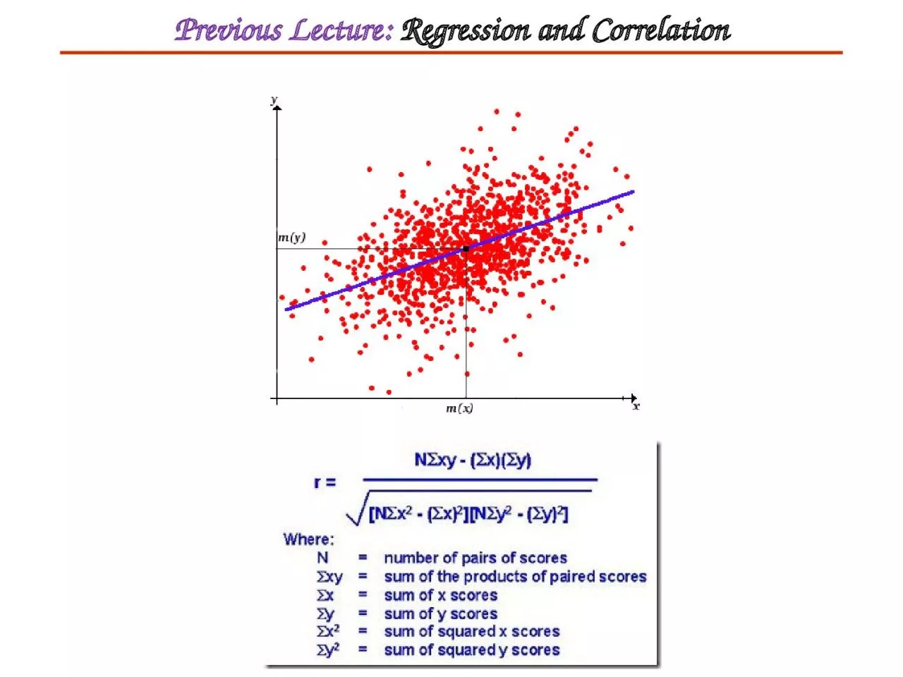
Previous Lecture:
Regression and Correlation
Slide2Introduction to Biostatistics and Bioinformatics
Proteomics Informatics
This Lecture
Slide3Proteomics Informatics – Learning Objectives
Structure of
m
ass spectrometry data
Protein identification
Protein quantitation
Slide4Protein Identification and Quantitation
by Mass Spectrometry
Mass
Spectrometry
m/z
intensity
Identity
Quantity
Samples
Peptides
Slide5Mass spectrometry
LysisFractionation
Sample preparation for protein identification, characterization and quantitation
Digestion
Slide6Overview of Mass spectrometry
Ion Source
Mass Analyzer
Detector
mass/charge
intensity
Slide7Mass Spectrometry (MS)
Slide8Example data – MALDI-TOF
Peptide intensity vs m/z
Slide9Peptide Fragmentation
Mass Analyzer 1
Frag-mentation
Detector
Ion Source
Mass Analyzer 2
b
y
Slide10Liquid Chromatography (LC)-MS/MS
Mass Analyzer 1
Frag-mentation
Detector
intensity
mass/charge
Ion Source
Mass Analyzer 2
LC
intensity
mass/charge
intensity
mass/charge
intensity
mass/charge
intensity
mass/charge
intensity
mass/charge
Time
intensity
mass/charge
intensity
mass/charge
intensity
mass/charge
intensity
mass/charge
intensity
mass/charge
intensity
mass/charge
intensity
mass/charge
intensity
mass/charge
intensity
mass/charge
Slide11Fragment intensity vs m/z
Example data – ESI-LC-MS/MS
Time
m/z
m/z
% Relative Abundance
100
0
250
500
750
1000
[M+2H]
2+
762
260
389
504
633
875
292
405
534
907
1020
663
778
1080
1022
MS/MS
Peptide intensity vs m/z vs time
Slide12Charge-State Distributions
mass/charge
intensity
MALDI
ESI
mass/charge
intensity
1+
1+
2+
3+
4+
Peptide
Protein
2+
M - molecular mass
n - number of charges
H – mass of a proton
mass/charge
intensity
mass/charge
intensity
1+
27+
2+
3+
4+
MALDI
ESI
5+
31+
Slide13Charge-State
Example:
peptide of mass 898 carrying 1 H+ = (898 + 1) / 1 = 899 m/z
carrying 2 H
+
= (898 + 2) / 2 = 450 m/z
carrying 3 H
+
= (898 + 3) / 3 = 300.3 m/z
M - molecular mass
n - number of charges
H – mass of a proton
Slide14Isotope Distributions
m/z
m/z
m/z
Intensity
0.015%
2
H
1.11%
13
C
0.366%
15
N
0.038%
17
O, 0.200%
18
O,
0.75%
33
S, 4.21%
34S, 0.02% 36
SOnly 12
C and 13C:p=0.0111n is the number of C in the peptidem is the number of
13C in the peptideTm is the relative intensity of the
peptide m 13C
12
C
14
N
16
O1H32S
+1Da
+2Da+3Da
Slide15Isotope Clusters and Charge State
m/z
Intensity
1+
1
1
1
m/z
Intensity
2+
0.5
0.5
0.5
m/z
Intensity
3+
0.33
0.33
0.33
Slide16432.8990
433.2330
433.5671
433.9014
713.3225
713.8239
714.3251
714.8263
What is the Charge State?
between the isotopes is 0.5
Da
between the isotopes is 0.33
Da
Slide17Protein Identification
by Mass Spectrometry
Mass
Spectrometry
m/z
intensity
Identity
Samples
Peptides
Slide18Protein Identification
- Exercise
1. Protein
identification: NUP1 was
genomically
tagged protein A, affinity purified under two conditions, and the resulting protein mixture was analyzed with liquid chromatography mass spectrometry (LC-MS). Search the resulting spectra (NUP1-less-stringent-wash.mgf, NUP1-more-stringent-wash.mgf) using X! Tandem (
http://h.thegpm.org/tandem/thegpm_tandem.html
). Change the taxon to “S.
cerevisiae
(budding yeast)” but otherwise keep the default parameter settings.
a. Look
at the list of identified proteins and explain why they are found in this sample. More information is also available by selecting the “go”, “path”, “
ppi
”, “
doms
”, “string” tabs on top of the page
.
b. Select the “
mh
” display on top right of the page, and zoom in to +/-100 ppm (the default setting for the mass accuracy that was used in the search). What precursor mass accuracy should we have used? Zoom in further and determine what precursor mass accuracy could have been used if the spectra were recalibrated (the error distribution centered at zero).
Slide19Identification – Tandem MS
Slide20m/z
% Relative Abundance
100
0
250
500
750
1000
Tandem MS – Sequence Confirmation
K
L
E
D
E
E
L
F
G
S
Slide21K
1166
L
1020
E
907
D
778
E
663
E
534
L
405
F
292
G
145
S
88
b ions
m/z
% Relative Abundance
100
0
250
500
750
1000
K
L
E
D
E
E
L
F
G
S
Tandem MS – Sequence Confirmation
Slide22147
K
1166
L
260
1020
E
389
907
D
504
778
E
633
663
E
762
534
L
875
405
F
1022
292
G
1080
145
S
1166
88
y ions
b ions
m/z
% Relative Abundance
100
0
250
500
750
1000
K
L
E
D
E
E
L
F
G
S
Tandem MS – Sequence Confirmation
Slide23147
K
1166
L
260
1020
E
389
907
D
504
778
E
633
663
E
762
534
L
875
405
F
1022
292
G
1080
145
S
1166
88
y ions
b ions
m/z
% Relative Abundance
100
0
250
500
750
1000
[M+2H]
2+
762
260
389
504
633
875
292
405
534
907
1020
663
778
1080
1022
K
L
E
D
E
E
L
F
G
S
Tandem MS – Sequence Confirmation
Slide24147
K
1166
L
260
1020
E
389
907
D
504
778
E
633
663
E
762
534
L
875
405
F
1022
292
G
1080
145
S
1166
88
y ions
b ions
m/z
% Relative Abundance
100
0
250
500
750
1000
[M+2H]
2+
762
260
389
504
633
875
292
405
534
907
1020
663
778
1080
1022
K
L
E
D
E
E
L
F
G
S
Tandem MS – Sequence Confirmation
Slide25147
K
1166
L
260
1020
E
389
907
D
504
778
E
633
663
E
762
534
L
875
405
F
1022
292
G
1080
145
S
1166
88
y ions
b ions
m/z
% Relative Abundance
100
0
250
500
750
1000
[M+2H]
2+
762
260
389
504
633
875
292
405
534
907
1020
663
778
1080
1022
113
K
L
E
D
E
E
L
F
G
S
113
Tandem MS – Sequence Confirmation
Slide26147
K
1166
L
260
1020
E
389
907
D
504
778
E
633
663
E
762
534
L
875
405
F
1022
292
G
1080
145
S
1166
88
y ions
b ions
m/z
% Relative Abundance
100
0
250
500
750
1000
[M+2H]
2+
762
260
389
504
633
875
292
405
534
907
1020
663
778
1080
1022
129
129
K
L
E
D
E
E
L
F
G
S
Tandem MS – Sequence Confirmation
Slide27Tandem MS – de novo Sequencing
m/z
% Relative Abundance
100
0
250
500
750
1000
[M+2H]
2+
762
260
389
504
633
875
292
405
534
907
1020
663
778
1080
1022
Mass Differences
Amino acid masses
Sequences
consistent
with spectrum
Slide28Tandem MS – de novo Sequencing
Slide29Tandem MS – de novo Sequencing
Slide30Tandem MS – de novo Sequencing
X
X
X
X
X
X
…GF(I/L)EEDE(I/L)…
…(I/L)EDEE(I/L)FG…
…GF(I/L)EEDE(I/L)…
…(I/L)EDEE(I/L)FG…
Peptide M+H = 1166
1166 -1079 = 87 => S
S
GF(I/L)EEDE(I/L)…
S
GF(I/L)EEDE(I/L)…
1166 – 1020 – 18 = 128
K or Q
SGF(I/L)EEDE(I/L)(
K/Q
)
Slide31Tandem MS – de novo Sequencing
Challenges in de novo sequencing
Neutral loss (-H2O, -NH3)
Modifications
Background peaks
Incomplete information
Challenges in de novo sequencing
Neutral loss (-H
2
O, -NH
3
)
Modifications
Background peaks
Incomplete information
Slide32MS/MS
Lysis
Fractionation
Tandem MS – Database Search
MS/MS
Digestion
Sequence
DB
All Fragment
Masses
Pick Protein
Compare, Score, Test Significance
Repeat for all proteins
Pick Peptide
LC-MS
Repeat for
all peptides
Slide33S.
cerevisiae
Human
Information Content in a Single Mass Measurement
Tryptic
peptide mass [
Da
]
1000 2000 3000
Tryptic
peptide mass [
Da
]
1000 2000 3000
Avg. #of matching peptides
#of matching peptides
1 2 3 4 6 8 10
10
8
6
4
3
2
1
Avg. #of matching peptides
10
8
6
4
3
2
1
#of matching peptides
1 2 3 4 6 8 10
Slide34Protein Identification and Quantitation
by Mass Spectrometry
Mass
Spectrometry
m/z
intensity
Quantity
Samples
Peptides
Slide35Fractionation
Digestion
LC-MS
Lysis
MS
Sample
i
Protein j
Peptide k
Protein Quantitation
by
Mass Spectrometry
Slide36Fractionation
Digestion
LC-MS
Lysis
Quantitation
– Label-Free (MS)
MS
MS
Assumption:
constant for all samples
Sample
i
Protein j
Peptide k
Slide37H
L
Quantitation – Metabolic Labeling
Fractionation
Digestion
LC-MS
Light
Heavy
Lysis
MS
Oda
et al. PNAS 96 (1999) 6591
Ong
et al. MCP 1 (2002) 376
Sample
i
Protein j
Peptide k
Slide38H
L
Fractionation
Digestion
LC-MS
Light
Lysis
Synthetic
Peptides
(Heavy)
Quantitation – Labeled Synthetic Peptides
MS
Gerber et al. PNAS 100 (2003) 6940
Enrichment with
Peptide antibody
Assumption: All losses after mixing are identical for the heavy and light isotopes and
Anderson
, N.L
., et
al.
Proteomics 3 (2004)
235-44
Slide39Estimating peptide quantity
Peak height
Curve fitting
Peak area
Peak height
Curve fitting
m/z
Intensity
Slide40What is the best way to estimate quantity?
Peak height - resistant to interference
- poor statisticsPeak area - better statistics
- more sensitive to interference
Curve fitting - better statistics
- needs to know the peak shape
- slow
Spectrum counting - resistant to interference
- easy to implement
- poor statistics for
low-abundance proteins
Slide41Proteomics Informatics - Summary
Structure of
m
ass spectrometry data
Protein identification
Protein quantitation
Slide42Next Lecture:
Gene Expression
Slide43Protein Quantitation - Exercise
2
. Protein quantitation: Two breast tumor
xenografts
(one basal and one luminal) were analyzed in by LC-MS and the spectral counts for the identified peptides in the different analyses are listed in two-sample-three-replicate-comparison.txt
.
a. Compare
replicate one of Sample 1 with replicate one of Sample 2 using proteomics_no_replicate.py. Which differences are significant
?
b. Compare replicate one and two of Sample 1 using proteomics_one_replicate.py. Compare to the distribution in 2a. Which differences are significant in 2a
?
c. Compare the three replicates of Sample 1 with the three replicates of Sample 2 using proteomics_three_replicates.py. Which differences are
significant
?
d. In cases when a protein is not observed in one sample, how many spectra do we need to observe in the other sample to say that there is a significant difference?
Slide44Phosphorylation Exercise: an unmodified peptide
Theoretical fragment ions
Slide45Spectrum of
the phosphorylated peptide
Slide46Spectrum of the peptide
phosphorylated at a different site