
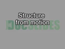
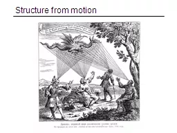
Camera 3 R 3 t 3 Figure credit Noah Snavely Camera 1 Camera 2 R 1 t 1 R 2 t 2 Structure from motion Camera 3 R 3 t 3 Camera 1 Camera 2 R 1 t 1 R 2 t 2 Structure ID: 782711
Download The PPT/PDF document "Multi-view geometry Structure from motio..." is the property of its rightful owner. Permission is granted to download and print the materials on this web site for personal, non-commercial use only, and to display it on your personal computer provided you do not modify the materials and that you retain all copyright notices contained in the materials. By downloading content from our website, you accept the terms of this agreement.


Slide1
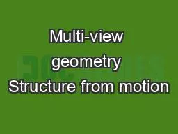
Multi-view geometry
Slide2Structure from motion
Camera 3
R
3
,t
3
Figure credit: Noah
Snavely
Camera 1
Camera 2
R
1
,t
1
R
2
,t
2
Slide3Structure from motion
Camera 3
R
3
,t
3
Camera 1
Camera 2
R
1
,t
1
R
2
,t
2
Structure:
Given
known cameras
and projections of the same 3D point in two or more images, compute the 3D coordinates of that point
?
Slide4Structure from motion
Camera 3
R
3
,t
3
Camera 1
Camera 2
R
1
,t
1
R
2
,t
2
Motion:
Given a set of
known
3D points seen by a camera, compute the camera parameters
?
?
?
Slide5Structure from motion
Camera 1
Camera 2
R
1
,t
1
R
2
,t
2
Bootstrapping the process:
Given a set of 2D point correspondences in
two images
, compute the camera parameters
?
?
Slide6Two-view geometry
Slide7Epipolar Plane
– plane containing baseline (1D family)
Epipoles
= intersections of baseline with image planes
= projections of the other camera center
= vanishing points of the motion direction
Baseline
– line connecting the two camera centers
Epipolar geometry
X
x
x’
Slide8The Epipole
Photo by Frank Dellaert
Slide9Epipolar Plane
– plane containing baseline (1D family)
Epipoles
= intersections of baseline with image planes
= projections of the other camera center
= vanishing points of the motion direction
Epipolar
Lines
- intersections of
epipolar
plane with image
planes (always come in corresponding pairs)
Baseline
– line connecting the two camera centers
Epipolar geometry
X
x
x’
Slide10Example 1
Converging cameras
Slide11Example 2
Motion parallel to the image plane
Slide12Example 3
Slide13Example 3
Motion is perpendicular to the image planeEpipole
is the “focus of expansion” and the principal point
Slide14Motion perpendicular to image plane
http://vimeo.com/48425421
Slide15Epipolar constraint
If we observe a point
x in one image, where can the corresponding point
x’
be in the other image?
x
x’
X
Slide16Potential matches for
x have to lie on the corresponding
epipolar
line
l
’.
Potential matches for x’ have to lie on the corresponding
epipolar line l.
Epipolar constraint
x
x’
X
x’
X
x’
X
Slide17Epipolar constraint example
Slide18X
x
x’
Epipolar constraint: Calibrated case
Intrinsic and extrinsic parameters of the cameras are known, world coordinate system is set to that of the first camera
Then the projection matrices are given by
K
[
I
| 0]
and
K
’[
R
|
t
]
We can multiply the projection matrices (and the image points) by the inverse of the calibration matrices to get
normalized
image coordinates:
Slide19X
x
x’ =
Rx+t
Epipolar constraint: Calibrated case
R
t
The vectors
Rx
,
t
, and
x’
are coplanar
=
(
x,
1)
T
Slide20Epipolar constraint: Calibrated case
X
x
x’ =
Rx+t
Recall:
The vectors
Rx
,
t
, and
x’
are coplanar
Slide21Epipolar constraint: Calibrated case
X
x
x’ =
Rx+t
Essential Matrix
(
Longuet
-Higgins, 1981)
The vectors
Rx
,
t
, and
x’
are coplanar
Slide22X
x
x’
Epipolar constraint: Calibrated case
E x
is the
epipolar
line associated with
x
(
l
' =
E x
)
Recall: a line is given by
ax + by + c
= 0
or
Slide23X
x
x’
Epipolar constraint: Calibrated case
E x
is the
epipolar
line associated with
x
(
l
' =
E x
)
E
T
x
'
is the
epipolar line associated with x'
(l =
ETx')
E e = 0 and ET
e' = 0E is singular (rank two)
E has five degrees of freedom
Slide24Epipolar constraint: Uncalibrated case
The calibration matrices K and K’
of the two cameras are unknownWe can write the epipolar
constraint in terms of
unknown
normalized coordinates:
X
x
x’
Slide25Epipolar constraint: Uncalibrated case
X
x
x’
Fundamental Matrix
(Faugeras and Luong, 1992)
Slide26Epipolar
constraint:
Uncalibrated case
F x
is the
epipolar
line associated with
x (l' = F x)
FTx' is the epipolar line associated with x'
(l = FTx')F e
= 0 and FTe' = 0
F is singular (rank two)F has seven degrees of freedom
X
x
x’
Slide27Estimating the fundamental matrix
Slide28The eight-point algorithm
Enforce rank-2 constraint (take SVD
of
F
and throw out the smallest singular value)
Solve homogeneous linear system using eight or more matches
Slide29Problem with eight-point algorithm
Slide30Problem with eight-point algorithm
Poor numerical conditioning
Can be fixed by rescaling the data
Slide31The normalized eight-point algorithm
Center the image data at the origin, and scale it so the mean squared distance between the origin and the data points is 2 pixelsUse the eight-point algorithm to compute
F from the normalized pointsEnforce the rank-2 constraint (for example, take SVD of
F
and throw out the smallest singular value)
Transform fundamental matrix back to original units: if
T
and T’ are the normalizing transformations in the two images, than the fundamental matrix in original coordinates is T’T F T
(Hartley, 1995)
Slide32Seven-point algorithm
Set up least squares system with seven pairs of correspondences and solve for null space (two vectors) using SVD Solve for linear combination of null space vectors that satisfies det(F)=0
Source: D.
Hoiem
Slide33Nonlinear estimation
Linear estimation minimizes the sum of squared algebraic distances between points x
’i and
epipolar
lines
F x
i (or points x
i and epipolar lines FTx’i):
Nonlinear approach: minimize sum of squared geometric distances
x
i
Slide34Comparison of estimation algorithms
8-point
Normalized 8-point
Nonlinear least squares
Av. Dist. 1
2.33 pixels
0.92 pixel
0.86 pixel
Av. Dist. 2
2.18 pixels
0.85 pixel
0.80 pixel
Slide35The Fundamental Matrix Song
http://
danielwedge.com/fmatrix
/
Slide36From epipolar geometry to camera calibration
Estimating the fundamental matrix is known as “weak calibration”If we know the calibration matrices of the two cameras, we can estimate the essential matrix: E
= K’T
FK
The essential matrix gives us the relative rotation and translation between the cameras, or their extrinsic parameters
Alternatively, if the calibration matrices are known, the
five-point algorithm
can be used to estimate relative camera pose