Schrödinger’s money: The strange marriage between - PowerPoint Presentation

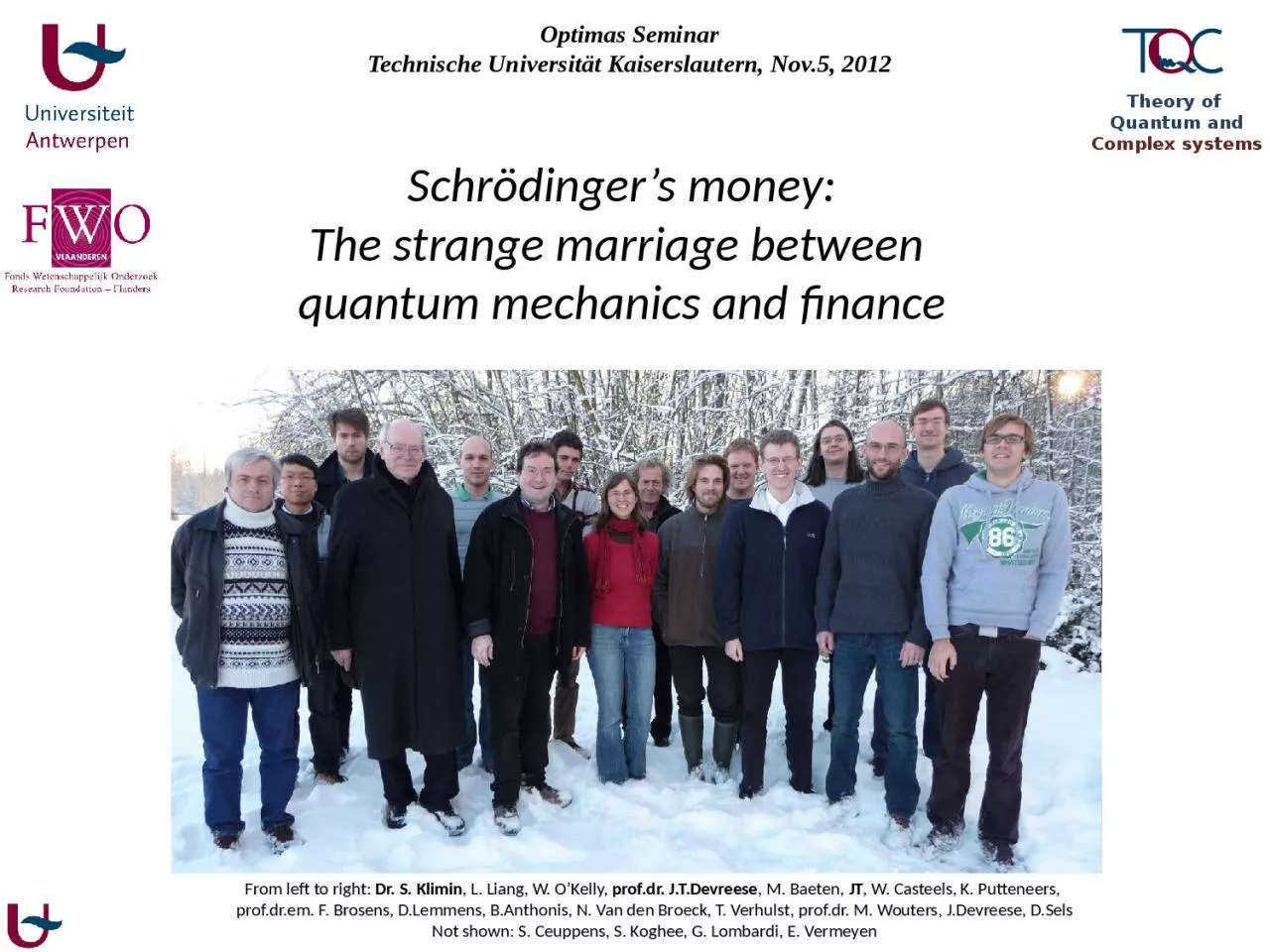
1. Schrödinger’s money:The strange marriage between quantum mechanics and financeFrom left to right: Dr. S. Klimin, L. Liang, W. O’Kelly, prof.dr. J.T.Devreese, M. Baeten, JT, W. Casteels, K. Putteneers, prof.dr.em. F. Brosens, D.Lemmens, B.Anthonis, N. Van den Broeck, T. Verhulst, prof.dr. M. Wouters, J.Devreese, D.SelsNot shown: S. Ceuppens, S. Koghee, G. Lombardi, E. VermeyenTheory of Quantum andComplex systemsOptimas SeminarTechnische Universität Kaiserslautern, Nov.5, 2012

2. Part I: path integrals in quantum mechanics

3. ABTwo alternatives: add the amplitudes12Introduction: quantum mechanics with path integrals

4. ABMany alternatives: add the amplitudesIntroduction: quantum mechanics with path integralsx

5. ABMany alternatives: add the amplitudesIntroduction: quantum mechanics with path integralsxt

6. ABMany alternatives: add the amplitudesIntroduction: quantum mechanics with path integralsxtx(t)The amplitude corresponding to a given path x(t) isHere, S is the action functional:With L the Lagrangian, eg. H. Kleinert, Path Integrals in Quantum Mechanics, Statistics, Polymer Physics, and Financial Markets, 5th ed. (World Scientific, Singapore, 2009)is called the path integral propagator

7. This prescription contains both classical mechanics (as a limit) : and “Schrödinger-picture” quantum mechanicsOnly when neighbouring paths have the same action functional will interfere constructively. H. Kleinert, Path Integrals in Quantum Mechanics, Statistics, Polymer Physics, and Financial Markets, 5th ed. (World Scientific, Singapore, 2009)

8. Introduction: Statistical mechanics with path integralsThe particle propagator or Green’s function as a Feynman path integral:The density matrix as a ‘Wiener’ path integralH. Kleinert, Path Integrals in Quantum Mechanics, Statistics, Polymer Physics, and Financial Markets, 5th ed. (World Scientific, Singapore, 2009)

9. Part II: Finance, and trading things in the future

10. Question #1 Choose between two rewards: (a) 100 € , one year from now (b) 100 € , right now Conclusion: Money now is worth more than money in the future.

11. Question #2 Choose between two rewards: (a) 100 € , one year from now (b) 0 € , right now Conclusion: Future money is worth something between 0% and 100% ofmoney now.Apply bracketing to find the amount where people find (a) and (b) equallyattractive.

12. At r = 0.02 , the value now of “100 euro one year from now” is 98.04 euro now. Homogeneous in time (“time consistency”): the preference of the options do not change when shifting both timesThe rational answer: discount the value at the interest rate for money savings.value( t + now) =value( t + a time T later)discounted valueExponentialdiscounting

13. Application to the student – beer relationshipReward 1: temporary Reward 2: no hangover lowering of social barrier the next dayAt this stage, the strategy “I will never drink again” wins.Here the strategy “What the heck, one more won’t hurt” has taken overvalue

14. value later: 100€value later: 0€probability q(T)probability 1-q(T)nowThe reason exponential discounting of future prices is not valid is RISKMain question in finance: how much is this ‘right to buy in the future’ worth?One year from now, you will require 100 tonne of steel; how do you deal with possible price fluctuations? 1. Decide a price now, say 630 EUR/tonne.A better deal (for you) is to buy the RIGHT, not the obligation to buy steel at 630 EUR/tonne one year from now.This is called an ‘option contract’. All types exist, eg.also the right to sell, with different times, and for different underlying assets.sT=730sT=530K=630s0=610

15. Size of derivatives market.CDS5 years of derivatives trading corresponds to a market equivalent to the total GDP of the human race since the beginning of civilization.Market value of all companies listed in stock exchanges:$45,000,000,000,000Banks: $7,000,000,000,000federal tax : 2.2 T$spending : 3.4 T$2011 data on money. Each block = 1000 billion dollar (1012 $)

16. Part III: Path integrals in finance

17. 1-p(T)p(T)1-p(T)p(T)1-p(T)p(T)1-p(T)p(T)Rather than 2 possible futures, there are many – but they can bee seen as a limit of many small ‘binomial’ steps  according to the central limit theorem, the outcome is Gaussian fluctuationsThe ‘standard model’ of option pricingp(T)1-p(T)p(T)1-p(T)p(T)1-p(T)p(T)1-p(T)p(T)1-p(T)p(T)1-p(T)Black-Scholes-Merton model:leads to exp{rT}cf. “exponential”discountingadds gaussianfluctuationsWe work with the logreturn to obtain This corresponds to a diffusion with diffusion constant 2 and drift (r2/2) per unit time.

18. 1-p(T)p(T)1-p(T)p(T)1-p(T)p(T)1-p(T)p(T)p(T)1-p(T)p(T)1-p(T)p(T)1-p(T)p(T)1-p(T)p(T)1-p(T)p(T)1-p(T)The ‘standard model’ of option pricingxAxxBRather than 2 possible futures, there are many – but they can bee seen as a limit of many small ‘binomial’ steps  according to the central limit theorem, the outcome is Gaussian fluctuationsThe probability to end up in xT is also given by the sum over all paths thatend up there, weighed by the probability of these pathsFrom the stochastic differential equationAn infinitesimal time-steppropagator is derived:xt

19. 1-p(T)p(T)1-p(T)p(T)1-p(T)p(T)1-p(T)p(T)p(T)1-p(T)p(T)1-p(T)p(T)1-p(T)p(T)1-p(T)p(T)1-p(T)p(T)1-p(T)The ‘standard model’ of option pricingxAxxBRather than 2 possible futures, there are many – but they can bee seen as a limit of many small ‘binomial’ steps  according to the central limit theorem, the outcome is Gaussian fluctuationsThe probability to end up in xT is also given by the sum over all paths thatend up there, weighed by the probability of these pathsxtFor the Black-Scholes model:From the stochastic differential equationAn infinitesimal time-steppropagator is derived:Many refs: Dash, Linetsky, Rosa-Clot, Kleinert,…

20. Black-Scholes-Merton and black mondayFisher Black & Myron Scholes, "The Pricing of Options and Corporate Liabilities". Journal of Political Economy 81 (3): 637–654 (1973).Robert C. Merton, "Theory of Rational Option Pricing“, Bell Journal of Economics and Management Science (The RAND Corporation) 4 (1): 141–183 (1973).Free particle propagator  Black-Scholes option priceRobert C. Merton Myron S. Scholes1997 nobel prize in economicsBoard members of “Long-Term Capital Management”,which initially made 40% return on investment as first users of the Black-Scholes model. Until in 1987 it lost all of its $4.6 billion.

21. Part IV: Beyond the standard model & the need for path integrals

22. Two problems with the standard modelProblem 2: Not all options have a payoff that depends only on x(t=T), many options have a path-dependentpayoff, i.e. payoff is a functional of x(t).Problem 1: The fluctuations are not GaussianΔxBlack-Scholes-Merton modelΔxFree particle propagator  Black-Scholes option price

23. Two problems with the standard modelProblem 2: Not all options have a payoff that depends only on x(t=T), many options have a path-dependentpayoff, i.e. payoff is a functional of x(t).Problem 1: The fluctuations are not GaussianFree particle propagator  Black-Scholes option pricep(T)1-p(T)p(T)1-p(T)p(T)p(T)1-p(T)p(T)1-p(T)p(T)1-p(T)1-p(T)p(T)1-p(T)p(T)1-p(T)xAxBxtAsian option: payoff is a function of the average of the underlying price?

24. Improving Black-Scholes : stochastic volatilityΔxBlack-Scholes-Merton modelΔxtHeston modelΔxtThe Heston model treats the variance as a second stochastic variable, satisfying its own stochastic differential equation:mean reversion ratemean reversion levelthe ‘volatility of the volatility’txtvtttwo particle problem

25. Improving Black-Scholes : stochastic volatilityΔxBlack-Scholes-Merton modelΔxtHeston modelΔxtUsing the prescription related before, the stochastic differential equations can be rewritten as an infinitesimal-time propagator, from which a Lagrangian can be identified(introducing z = (v/)1/2 ) :txtvtttwo particle problemthe transition probability for a price and volatility to go from x0,z0 at time t=0 to xT,zT at T (details: D.Lemmens, M. Wouters, JT, S. Foulon, Phys. Rev. E 78, 016101 (2008)).

26. Other improvements to Black-ScholesA) Stochastic Volatility* Heston model:* Hull-White model* Exponential Vasicek modelB) Jump Diffusion (and Levy models)poisson processBSAdd stoch vol. Add jump diff.HestonKouagain a zoo of proposalsH. Kleinert , Option Pricing from Path Integral for Non-Gaussian Fluctuations.Natural Martingale and Application to Truncated Lévy Distributions , Physica A 312, 217 (2002).

27. Other models and other tricksImprovements to Black-Scholes ...translate into ...to which quantum mechanics physical actions solving techniques can be appliedA) Stochastic Volatility 1. Heston model free particle coupled to exact solution radial harmonic oscillatorB) Stochastic volatiltiy + Jump Diffusion2. Exponential Vasicek model particle in an exponential perturbational gauge field generated by (Nozieres – Schmitt-Rink free particle expansion)3. Kou and Merton’s models particle in complicated variational (Jensen-Feynman potential (not previously variational principle) studied)References1. D. Lemmens, M. Wouters, J. Tempere, S. Foulon, Phys. Rev. E 78 (2008) 016101.2. L. Z. Liang, D. Lemmens, J. Tempere, European Physical Journal B 75 (2010) 335–342.3. D. Lemmens, L. Z. J. Liang, J. Tempere, A. D. Schepper, Physica A 389 (2010) 5193 – 5207.

28. More complicated payoffs‘Plain vanilla’ or simple options have a payoff that only depends on the value of the underlying at expiration, x(t=T). For such options we have:Many other option contracts have a payoff that depends on the entire path, such as:Asian options: payoff depends on the average price during the option lifetimeTimer options: contract duration depends on a volatility budgetBarrier options: contract becomes void if price goes above/below some valueFor such options, the price is given byFeynman-Kac ‘interpretation’  include payoff in the path weight:

29. ConclusionstStFluctuating paths in finance are described by stochastic models, which can be translated to Lagrangians for path integration.Path integrals can solve in a unifying framework the two problems of the ‘standard model of finance’:1/ The real fluctuations are not gaussian 2/ New types of option contracts have path- dependent payoffsD. Lemmens, M. Wouters, JT, S. Foulon, Phys. Rev. E 78, 016101 (2008); J.P.A. Devreese, D. Lemmens, JT, Physica A 389, 780-788 (2010);L. Z. J. Liang, D. Lemmens, JT, European Physical Journal B 75, 335–342 (2010); L. Z. J. Liang, D. Lemmens, JT, Physical Review E 83, 056112 (2011).D. Lemmens, L. Z. J. Liang, JT, A. D. Schepper, Physica A 389, 5193–5207 (2010);

30. Closing remark #1How can we choose between the zoo of models? Various models have been proposed to include various properties, or specific characteristic of financial time series, such as: * short memory of the returns * long memory of the volatility * heavy-tails in the return distribution * jumps * scale-free behavior of logreturns near crashApproach A: Superstatistics to discriminate between stochastic volatility modelsApproach B: Game theory on scale-free networks as microscopic theory to generate time series Link to physics:Ising models for2-state objectsinteracting on a lattice.(2 states: buy andsell; price is anemergent property)Ising parametersgiven by the Nash table fromminority gamesa method to “deconvolute” the underlying distribution of volatilities from the time seriesscale-free networksare more realistic than regular or randomlattices

31. Closing remark #2“I don’t believe talks about econophysics at conferences. Physicists who really worked out a predictive model of the market won’t be found at conferences. They’d be on some tropicalisland keeping quiet about it.” (Larry Schulman, path integral conference Antwerpen 1999)“Econophysics cannot tell you when exactly the market will crash, just like elasticity theory and tribology cannot predict where exactly on the mountain you will fall if you climb it using beach slippers. Nevertheless elasticity theory and tribology have a lot to say about beach slippers.”(Eugene Stanley, APS March meeting 2008)What ‘econophysics’ is not

32.

33. Additional material

34. More complicated payoffs Other example: Timer options in the Heston framework Timer options have an uncertain expiry time, equal to the time at which a certain “variance budget” has been used up)L. Z. J. Liang, D. Lemmens, and J. Tempere, Physical Review E 83, 056112 (2011).A Duru-Kleinert transformation allows to introduced a warped spacetime, linking real time and variance budget. This results in a particle in a Kratzer potential, allowing an exact solution.

35. More complicated payoffs Other example: Timer options in the Heston framework Timer options have an uncertain expiry time, equal to the time at which a certain “variance budget” has been used up)L. Z. J. Liang, D. Lemmens, and J. Tempere, Physical Review E 83, 056112 (2011).The probability density function for a given dose D to be reached at time TD, as a function of TD. The colours correspond to D = 10, .., 60 in steps of 10.Leads also to new formulas for estimating the maximum exposure time in an environment with fluctuating radioactivity

36. 1-p(T)p(T)1-p(T)p(T)1-p(T)p(T)1-p(T)p(T)The ‘standard model’ of option pricingp(T)1-p(T)p(T)1-p(T)p(T)1-p(T)p(T)1-p(T)p(T)1-p(T)p(T)1-p(T)Black-Scholes-Merton model:leads to exp{rT}cf. “exponential”discountingadds gaussianfluctuationsWhat is the transition probability for a price to go from xa at time ta to xb at tb ?Dash, Linetsky, Rosa-Clot, Kleinert,…

37. Calculating the path integral: time slicingrra(t0)timet0 rb(t)ttjtj-1

38. Path integrals and the polaronProf.dr. Widera’s research group:probing Cs atoms in Rb condensateUltracold gases are used as a quantum simulator to model the polaronJT, W. Casteels, M. K. Oberthaler, S. Knoop, E. Timmermans, and J. T. Devreese, Phys. Rev. B 80, 184504 (2009); W. Casteels, JT, J.T.Devreese, Phys. Rev. A 83, 033631 (2011).

39. Hyperbolic discountingExponentialdiscountingvalue

40. Compare:Do you prefer: (a) 100’000 € in 21 years (b) 98’039 € in 20 yearstoDo you prefer: (a) 100’000 € in 1 year (b) 98’039 € nowThe most prominent choiceThe most prominent choice Human psychology does not work with exponential discounting

41. Improving Black-Scholes : stochastic volatilityFor the uncorrelated system, it is worth simplifying the notation again, and introducing z = (v/)1/2 .What is the transition probability for a price and volatility to go from x0,z0 at time t=0 to xT,zT at T ?time-slicing + gaussian integrations{t1,x1,z1},…,{tN-1,xN-1,zN-1}D. Lemmens, M. Wouters, JT, S. Foulon, Phys. Rev. E 78, 016101 (2008).

42. AB Classical: add the probabilities12Introduction: quantum mechanics with path integrals

43. Improving Black-Scholes : stochastic volatilityFor the uncorrelated system, it is worth simplifying the notation again, and introducing z = (v/)1/2 .What is the transition probability for a price and volatility to go from x0,z0 at time t=0 to xT,zT at T ?=D. Lemmens, M. Wouters, JT, S. Foulon, Phys. Rev. E 78, 016101 (2008).