
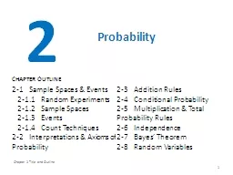
1 2 Probability 21 Sample Spaces amp Events 211 Random Experiments 212 Sample Spaces 213 Events 214 Count Techniques 22 Interpretations amp Axioms of Probability ID: 258539
Download Presentation The PPT/PDF document "Chapter 2 Title and Outline" is the property of its rightful owner. Permission is granted to download and print the materials on this web site for personal, non-commercial use only, and to display it on your personal computer provided you do not modify the materials and that you retain all copyright notices contained in the materials. By downloading content from our website, you accept the terms of this agreement.


Slide1
Chapter 2 Title and Outline
1
2
Probability
2-1 Sample Spaces & Events 2-1.1 Random Experiments 2-1.2 Sample Spaces 2-1.3 Events 2-1.4 Count Techniques2-2 Interpretations & Axioms of Probability2-3 Addition Rules2-4 Conditional Probability2-5 Multiplication & Total Probability Rules2-6 Independence2-7 Bayes’ Theorem2-8 Random Variables
CHAPTER OUTLINESlide2
2
Chapter 2 Learning Objectives
© John Wiley & Sons, Inc.
Applied Statistics and Probability for Engineers, by Montgomery and Runger.
Learning Objectives for Chapter 2After careful study of this chapter, you should be able to do the following:Understand and describe sample spaces and events for random experiments with graphs, tables, lists, or tree diagrams.Interpret probabilities and use probabilities of outcomes to calculate probabilities of events in discrete sample spaces.
Use permutation and combinations to count the number of outcomes in both an event and the sample space .
Calculate the probabilities of joint events such as unions and intersections from the probabilities of individuals events.
Interpret and calculate conditional probabilities of events.
Determine the independence of events and use independence to calculate probabilities.
Use Bayes’ theorem to calculate conditional probabilities .
Understand random variables.Slide3
Random Experiments
3
Sec 2-1.1 Random Experiments
Figure 2-1 Continuous iteration between model and physical system.
The goal is to understand, quantify and model the variation affecting a physical system’s behavior. The model is used to analyze and predict the physical system’s behavior as system inputs affect system outputs. The predictions are verified through experimentation with the physical system.Slide4
Noise Produces Output Variation
Sec 2-1.1 Random Experiments
4
Figure 2-2
Noise variables affect the transformation of inputs to outputs.Random values of the noise variables cannot be controlled and cause the random variation in the output variables. Holding the controlled inputs constant does not keep the output values constant.Slide5
Random Experiment
An experiment is an operation or procedure, carried out under controlled conditions, executed to discover an unknown result or to illustrate a known law.An experiment that can result in different outcomes, even if repeated in the same manner every time, is called a
random experiment.Sec 2-1.1 Random Experiments
5Slide6
Randomness Affects Natural Law
Sec 2-1.1 Random Experiments
6
Figure 2-3
A closer examination of the system identifies deviations from the model.Ohm’s Law current is a linear function of voltage. However, current will vary due to noise variables, even under constant voltage.Slide7
Randomness Can Disrupt a System
Telephone systems must have sufficient capacity (lines) to handle a random number of callers at a random point in time whose calls are of a random duration.
If calls arrive exactly every 5 minutes and last for exactly 5 minutes, only 1 line is needed – a deterministic system.Practically, times between calls are random and the call durations are random. Calls can come into conflict as shown in following slide.Conclusion: Telephone system design must include provision for input variation.
Sec 2-1.1 Random Experiments7Slide8
Deterministic & Random Call Behavior
Sec 2-1.1 Random Experiments
8
Figure 2-4
Variation causes disruption in the system.Calls arrive every 5 minutes. In top system, call durations are all of 5 minutes exactly. In bottom system, calls are of random duration, averaging 5 minutes, which can cause blocked calls, a “busy” signal.Slide9
Sample Spaces
Random experiments have unique outcomes.
The set of all possible outcome of a random experiment is called the sample space, S.S is discrete
if it consists of a finite or countable infinite set of outcomes.S is continuous if it contains an interval (either a finite or infinite width) of real numbers.
Sec 2-1.2 Sample Spaces9Slide10
Example 2-1: Defining Sample Spaces
Randomly select and measure the thickness of a part. S =
R+ = {x|x > 0}, the positive real line. Negative or zero thickness is not possible. S is continuous.
It is known that the thickness is between 10 and 11 mm. S = {x|10 < x < 11}, continuous.
It is known that the thickness has only three values. S = {low, medium, high}, discrete.Does the part thickness meet specifications? S = {yes, no}, discrete.Sec 2-1.2 Sample Spaces10Slide11
Example 2-2: Defining Sample Spaces, n=2
Two parts are randomly selected & measured. S
= R+ * R+, S is continuous.Do the 2 parts conform to specifications?
S = {yy, yn, ny, nn}, S is discrete.Number of conforming parts?
S = {1, 1, 2}, S is discrete.Parts are randomly selected until a non-conforming part is found. S = {n, yn, yyn, yyyn, …}, S is countably infinite.Sec 2-1.2 Sample Spaces11Slide12
Sample Space Is Defined By A Tree Diagram
Sec 2-1.2 Sample Spaces
12Example 2-3
: Messages are classified as on-time or late. 3 messages are classified. There are 23 = 8 outcomes in the sample space. S = {ooo, ool,olo, oll, loo, lol, llo, lll}
Figure 2-5 Tree diagram for three messages.Slide13
Tree Diagrams Can Fit The Situation
Sec 2-1.2 Sample Spaces
13
Example 2-4: New cars can be equipped with selected options as follows:
Manual or automatic transmissionWith or without air conditioningThree choices of stereo sound systemsFour exterior color choicesFigure 2-6 Tree diagram for different configurations of vehicles. Note that S has 2*2*3*4 = 48 outcomes.Slide14
Tree Diagrams Help Count Outcomes
Sec 2-1.2 Sample Spaces, Figure 2-7.
14
Example 2-5: The interior car color can depend on the exterior color as shown in the tree diagrams below. There are 12 possibilities without considering color combinations.
Figure 2-7 Tree diagram for different vehicle configurations with interior colors.Slide15
Events Are Sets of Outcomes
An event (E) is a subset of the sample space of a random experiment, i.e., one or more outcomes of the sample space.
Event combinations are:Union of two events is the event consisting of all outcomes that are contained in either of two events, E1
E2. Called E1 or E
2.Intersection of two events is the event consisting of all outcomes that contained in both of two events, E1 E2. Called E1 and E2.
Complement
of an event is the set of outcomes that are
not
contained in the event, E’ or
not
E.
Sec 2-1.3 Events
15Slide16
Example 2-6, Discrete Event Algebra
Recall the sample space from Example 2-2, S
= {yy, yn, ny, nn} concerning conformance to specifications.Let E1 denote the event that at least one part does conform to specifications, E
1 = {yy, yn, ny}Let E2 denote the event that no part conforms to specifications, E
2 = {nn}Let E3 = Ø, the null or empty set.Let E4 = S, the universal set.Let E5 = {yn, ny, nn
}, at least one part
does not
conform.
Then E
1
E
5
=
S
Then E
1
E
5
= {
yn, ny
}
Then E
1
’
= {
nn
}
Sec 2-1.3 Events
16Slide17
Example 2-7, Continuous Event Algebra
Measurements of the thickness of a part are modeled with the sample space:
S = R+.Let E1 = {x|10 ≤ x
< 12}, show on the real line below.Let E2 = {x|11 < x
< 15}Then E1 E2 = {x|10 ≤ x < 15}Then E1 E2
=
{
x
|11 <
x
< 12}
Then E
1
’ = {
x
|
x
< 10 or
x
≥ 12}
Then E
1
’
E
2
=
{
x
|12 ≥
x
< 15}
Sec 2-1.2 Sample Spaces
17Slide18
Example 2-8, Hospital Emergency Visits
This table summarizes the ER visits at 4 hospitals. People may leave without being seen by a physician( LWBS). The remaining people are seen, and may or may not be admitted.
Let A be the event of a visit to Hospital 1.Let B be the event that the visit is LWBS.Find number of outcomes in:
A BA’
A BSec 2-1.2 Sample Spaces18Slide19
Venn Diagrams Show Event Relations
Sec 2-1.3 Events
19
Events A & B contain their respective outcomes. The shaded regions indicate the event relation of each diagram.
Figure 2-8 Venn diagramsSlide20
Venn Diagram of Mutually Exclusive Events
Sec 2-1.3 Events
20
Events A & B are mutually exclusive because they share no common outcomes.The occurrence of one event precludes the occurrence of the other. Symbolically, A B = ØFigure 2-9 Mutually exclusive eventsSlide21
Event Relation Laws
Transitive law (event order is unimportant): A
B = B A and A B = B
ADistributive law (like in algebra): (A
B) C = (A C) (B C) (A B) C = (A
C)
(B
C)
DeMorgan’s laws:
(
A
B)’ =
A’
B’ The complement of the union is the intersection of the complements.
(
A
B)’ =
A’
B’ The complement of the intersection is the union of the complements.
Sec 2-1.3 Events
21Slide22
Counting Techniques
These are three special rules, or counting techniques, used to determine the number of outcomes in the events and the sample space.They are the:
Multiplication rulePermutation ruleCombination ruleEach has its special purpose that must be applied properly – the right tool for the right job.
Sec 2-1.4 Counting Techniques
22Slide23
Counting – Multiplication Rule
Multiplication rule:Let an operation consist of k steps and
n1 ways of completing step 1,n2 ways of completing step 2, … andnk ways of completing step k.
Then, the total number of ways or outcomes are:n1 * n2*…*n
k Sec 2-1.4 Counting Techniques23Slide24
Example 2-9: Multiplication Rule
In the design for a gear housing, we can choose to use among: 4 different fasteners, 3 different bolt lengths and
2 different bolt locations.How many designs are possible?Answer: 4 * 3 * 2 = 24Sec 2-1.4 Counting Techniques
24Slide25
Counting – Permutation Rule
A permutation is a unique sequence of distinct items.
If S = {a, b, c}, then there are 6 permutations Namely: abc, acb, bac, bca, cab, cba (order matters)The # of ways 3 people can be arranged.
# of permutations for a set of n items is n!n! (factorial function) = n*(n-1)*(n-2)*…*2*17! = 7*6*5*4*3*2*1 = 5,040 = FACT(7) in ExcelBy definition: 0! = 1
Sec 2-1.4 Counting Techniques25Slide26
Counting – Sub-set Permutations
To sequence only r items from a set of n items:
Sec 2-26Slide27
Example 2-10: Circuit Board Designs
A printed circuit board has eight different locations in which a component can be placed. If four different components are to be placed on the board , how many designs are possible?Answer: order is important, so use the permutation formula with n = 8, r = 4.
Sec 2-1.4 Counting Techniques
27Slide28
Counting - Similar Item Permutations
Used for counting the sequences when not all the items are different.The number of permutations of:
n = n1 + n2 + … + nr items of which n1 are identical,
n2 are identical, … , and nr are identical.
Is calculated as:Sec 2-1.4 Counting Techniques28Slide29
Example 2-11: Machine Shop Schedule
In a machining operation, a piece of sheet metal needs two identical-diameter holes drilled and two identical-size notched cut. The drilling operation is denoted as d and the notching as n.
How many sequences are there? What is the set of sequences? {ddnn, dndn, dnnd, nddn, ndnd, nndd}
Sec 2-1.4 Counting Techniques29Slide30
Example 2-12: Bar Codes
A part is labeled with 4 thick lines, 3 medium lines, and two thin lines. Each sequence is a different label.How many unique labels can be created?
In Excel:Sec 2-1.4 Counting Techniques
30Slide31
Counting – Combination Rule
A combination is a selection of r items from a set of n where
order does not matter.If S = {a, b, c}, n =3, then there is 1 combination. If r =3, there is 1 combination, namely: abc If r=2, there are 3 combinations, namely ab, ac, bc
# of permutations ≥ # of combinationsSec 2-1.4 Counting Techniques
31Slide32
Example 2-13: Applying the Combination Rule
A circuit board has eight locations in which a component can be placed. If 5 identical components are to be placed on a board, how many different designs are possible?
The order of the components is not important, so the combination rule is appropriate.Excel:Sec 2-1.4 Counting Techniques
32Slide33
Example 2-14: Sampling w/o Replacement-1
A bin of 50 parts contains 3 defectives & 47 good parts. A sample of 6 parts is selected from the 50
without replacement.How many different samples of size 6 are there that contain exactly 2 defective parts?In Excel:
Sec 2-1.4 Counting Techniques33Slide34
Example 2-14: Sampling w/o Replacement-2
Now, how many ways are there of selecting 4 parts from the 47 acceptable parts?
In Excel:Sec 2-1.4 Counting Techniques
34Slide35
Example 2-14: Sampling w/o Replacement-3
Now, how many ways are there to obtain:2 from the 3 defectives,
and4 from the 47 non-defectives?In Excel:
Sec 2-1.4 Counting Techniques35Slide36
Example 2-14: Sampling w/o Replacement-4
Furthermore, how many ways are there to obtain 6 parts (0-6 defectives) from the set of 50?
So the ratio of obtaining 2 defectives out 6 to any number (0-6) defectives out of 6 is:Sec 2-1.4 Counting Techniques
36Slide37
What Is Probability?
Probability is the likelihood or chance that a particular outcome or event from a random experiment will occur.
Here, only finite sample spaces ideas apply.Probability is a number in the [0,1] interval.May be expressed as a: proportion (0.15) percent (15%) fraction (3/20)A probability of:
1 means certainty 0 means impossibilitySec 2-2 Interpretations & Axioms of Probability
37Slide38
Types of Probability
Subjective probability
is a “degree of belief.”“There is a 50% chance that I’ll study tonight.”Relative frequency probability is based how often an event occurs over a very large sample space.
Sec 2-2 Interpretations & Axioms of Probability
38Figure 2-10 Relative frequency of corrupted pulses over a communications channelSlide39
Probability Based on Equally-Likely Outcomes
Whenever a sample space consists of N
possible outcomes that are equally likely, the probability of each outcome is 1/N.Example: In a batch of 100 diodes, 1 is colored red. A diode is randomly selected from the batch. Random means each diode has an equal chance of being selected. The probability of choosing the red diode is 1/100 or 0.01, because each outcome in the sample space is equally likely.
Sec 2-2 Interpretations & Axioms of Probabilities39Slide40
Example 2-15: Laser Diodes
Assume that 30% of the laser diodes in a batch of 100 meet a customer requirements.
A diode is selected randomly. Each diode has an equal chance of being selected. The probability of selecting an acceptable diode is 0.30.
Sec 2-2 Interpretations & Axioms of Probability40
Figure 2-11 Probability of the event E is the sum of the probabilities of the outcomes in E.Slide41
Probability of an Event
For a discrete sample space, the probability of an event E, denoted by
P(E), equals the sum of the probabilities of the outcomes in E.The discrete sample space may be: A finite set of outcomes A countably infinite set of outcomes.Further explanation is necessary to describe probability with respect to continuous sample spaces.
Sec 2-2 Interpretations & Axioms of Probability
41Slide42
Example 2-16: Probabilities of Events
A random experiment has a sample space {w,x,y,z}. These outcomes are
not equally-likely; their probabilities are: 0.1, 0.3, 0.5, 0.1.Event A ={w,x}, event B = {x,y,z}, event C = {z}
P(A) = 0.1 + 0.3 = 0.4P(B) = 0.3 + 0.5 + 0.1 = 0.9 P(C) = 0.1
P(A’) = 0.6 and P(B’) = 0.1 and P(C’) = 0.9 Since event AB = {x}, then P(AB) = 0.3 Since event AB = {w,x,y,z
}, then P(
A
B) = 1.0
Since event
A
C = {null}, then P(
A
C ) = 0.0
Sec 2-2 Interpretations & Axioms of Probability
42Slide43
Example 2-17: Contamination Particles
An inspection of a large number of semiconductor wafers revealed the data for this table. A wafer is selected randomly.
Sec 2-2 Interpretations & Axioms of Probability43
Let E be the event of selecting a 0 particle wafer. P(E) = 0.40
Let E be the event of selecting a wafer with 3 or more particles. P(E) = 0.10+0.05+0.10 = 0.25Slide44
Example 2-18: Sampling w/o Replacement
A batch of parts contains 6 parts {a,b,c,d,e,f
}. Two are selected at random. Suppose part f is defective. What is the probability that part f appears in the sample?How many possible samples can be drawn?Excel:How many samples contain part f? 5 by enumeration: {
af,bf,cf,df,ef}P(defective part) = 5/15 = 1/3.
Sec 2-2 Interpretations & Axioms of Probability44Slide45
Axioms of Probability
Probability is a number that is assigned to each member of a collection of events from a random experiment that satisfies the following properties:
P(S) = 10 ≤ P(E) ≤ 1For each two events
E1 and E2 with E
1E2 = Ø, P(E1E2) = P(E
1
)
+
P(E
2
)
These imply that:
P(
Ø)
=0 and
P(E’)
= 1 –
P(E)
If
E
1
is contained in
E
2
, then
P(E
1
)
≤
P(E
2
)
.
Sec 2-2 Interpretations & Axioms of Probability
45Slide46
Addition Rules
Joint events are generated by applying basic set operations to individual events, specifically:Unions of events,
A BIntersections of events, A
BComplements of events, A’Probabilities of joint events can often be determined from the probabilities of the individual events that comprise it. And conversely.
Sec 2-3 Addition Rules46Slide47
Example 2-19: Semiconductor Wafers
A wafer is randomly selected from a batch as shown in the table.
Let H be the event of high concentrations of contaminants. Then P(H) = 358/940.Let C be the event of the wafer being located at the center of a sputtering tool used in manufacture. Then P(
C) = 626/940.P(HC
) = 112/940P(HC) = P(H) + P
(
C
) -
P
(
H
C
) = (358+626-112)/940 This is the
addition rule
.
Sec 2-3 Addition Rules
47Slide48
The probability of a union:
If events A and B are mutually exclusive:
Sec 2-3 Addition Rules48Slide49
Example 2-20: Contaminants & Location
Wafers in last example are now classified by degree of contamination per table of proportions.
Sec 2-3 Addition Rules
49
E1 is the event that a wafer has 4 or more particles. P(E1) = 0.15 E2 is the event that a wafer was on edge.
P
(
E
2
) = 0.28
P
(
E
1
E
2
) = 0.04
P
(
E
1
E
2
)
=0.15 + 0.28 – 0.04
= 0.39Slide50
Addition Rule: 3 or More Events
Sec 2-3 Addition Rules
50
(2-7)
Note the alternating signs.(2-8)Slide51
Venn Diagram of Mutually Exclusive Events
Sec 2-3 Addition Rules, Figure 2-12
51
Figure 2-12
Venn diagram of four mutually exclusive events. Note that no outcomes are common to more than one event, i.e. all intersections are null.Slide52
Example 2-21: pH
Let X denote the pH of a sample. Consider the event that P(6.5 < X
≤ 7.5) = P(6.5 < X ≤ 7.0) + P(7.0 < X ≤ 7.5) +
P(7.5 < X ≤ 7.8)The partition of an event into mutually exclusive subsets is widely used to allocate probabilities.
Sec 2-3 Addition Rule52Slide53
Conditional Probability
Probabilities should be reevaluated as additional information becomes available.
P(B|A) is called the probability of event B occurring, given that event A has already occurred.
A communications channel has an error rate of 1 per 1000 bits transmitted. Errors are rare, but do tend to occur in bursts. If a bit is in error, the probability that the next bit is also an error ought to be greater than 1/1000.Sec 2-4 Conditional Probability
53Slide54
An Example of Conditional Probability
In a thin film manufacturing process, the proportion of parts that are not acceptable is 2%. However the process is sensitive to contamination that can increase the rate of parts rejection.If we know that the plant is having filtration problems that increase film contamination, we would presume that the rejection rate has increased.
Sec 2-4 Conditional Probability
54Slide55
Another Example of Conditional Probability
Sec 2-4 Conditional Probability
55
Figure 2-13
Conditional probability of rejection for parts with surface flaws and for parts without surface flaws. The probability of a defective part is not evenly distributed. Flawed parts are five times more likely to be defective than non-flawed parts, i.e., P(D|F) / P(D|F’).Slide56
Example 2-22: A Sample From Prior Graphic
Table 2-3 shows that 400 parts are classified by surface flaws and as functionally defective. Observe that:
P(D|F) = 10/40 = 0.25 P
(D|F’) = 18/360 = 0.05
Sec 2-4 Conditional Probability56Slide57
Conditional Probability Rule
The conditional probability of event
B given event A, denoted as P(A|B), is:
P(B|A) = P(A
B) / P(A) (2-9)for P(A) > 0.From a relative frequency perspective of n equally likely outcomes:P
(
A
) = (number of outcomes in
A
) / n
P(
A
B
) = (number of outcomes in
A
B
)
/ n
Sec 2-4 Conditional Probability
57Slide58
Example 2-23: More Surface Flaws
Refer to Table 2-3 again. There are 4 probabilities conditioned on flaws.
Sec 2-4 Conditional Probability58Slide59
Example 2-23: Tree Diagram
Sec 2-4 Conditional Probability
59
Figure 2-14
Tree diagram for parts classificationTree illustrates sampling two parts without replacement: At the 1st stage (flaw), every original part of the 400 is equally likely. At the 2nd stage (defect), the probability is conditional upon the part drawn in the prior stage.Slide60
Random Samples & Conditional Probabilities
Random means each item is equally likely to be chosen. If more than one item is sampled, random means that every sampling outcome is equally likely.
2 items are taken from S = {a,b,c} without replacement.Ordered sample space: S = {ab,ac,bc,ba,bc,cb
}Unordered sample space: S = {ab,ac,bc}This is done by enumeration – too hard
Sec 2-4 Conditional Probability60Slide61
Sampling Without Enumeration
Use conditional probability to avoid enumeration. To illustrate: A batch of 50 parts contains 10 made by Tool 1 and 40 made by Tool 2. We take a sample of n=2.
What is the probability that the 2nd part came from Tool 2, given that the 1st part came from Tool 1? P(1st part came from Tool 1) = 10/50
P(2nd part came from Tool 2) = 40/49P(Tool 1, then Tool 2 part sequence) = (10/50)*(40/49)To select randomly implies that, at each step of the sample, the items remaining in the batch are equally likely to be selected.
Sec 2-4 Conditional Probability61Slide62
Example 2-24: Sampling Without Replacement
A production lot of 850 parts contains 50 defectives. Two parts are selected at random.
What is the probability that the 2nd is defective, given that the first part is defective?Let A denote the event that the 1st part selected is defective.Let
B denote the event that the 2nd part selected is defective.Probability desired is P(
B|A) = 49/849.Sec 2-4 Conditional Probability62Slide63
Example 2-25: Continuing Prior Example
Now, 3 parts are sampled randomly.What is the probability that the first two are defective, while the third is not?
In Excel:Sec 2-4 Conditional Probability
63Slide64
Multiplication Rule
The conditional probability definition of Equation 2-9 can be rewritten to generalize it as the multiplication
rule.P(AB) = P
(B|A)*
P(A) = P(A|B)*P(B) (2-10)The last expression is obtained by exchanging the roles of
A
and
B
.
Sec 2-5 Multiplication & Total Probability Rules
64Slide65
Example 2-26: Machining Stages
The probability that, a part made in the 1st stage of a machining operation passes inspection, is 0.90. The probability that, it passes inspection after the 2
nd stage, is 0.95.What is the probability that the part meets specifications?Let A & B denote the events that the 1st & 2nd stages meet specs.
P(AB) =
P(B|A)*P(A) = 0.95*0.90 = 0.955Sec 2-65Slide66
Two Mutually Exclusive Subsets
Sec 2-5 Multiplication & Total Probability Rules
66
Figure 2-15
Partitioning an event into two mutually exclusive subsets. A & A’ are mutually exclusive. AB and A’
B
are mutually exclusive
B
= (
A
B
)
(
A
B
)Slide67
Total Probability Rule
For any two events A and B
:Sec 2-5 Multiplication & Total Probability Rules
67Slide68
Example 2-27: Semiconductor Contamination
Information about product failure based on chip manufacturing process contamination.
F denotes the event that the product fails. H denotes the event that the chip is exposed to high contamination during manufacture.
P(F|H) = 0.100 & P
(H) = 0.2, so P(FH) = 0.02P(F|H’) = 0.005 and P(H’) = 0.8, so P(
F
H’
) = 0.004
P
(
F
) =
P
(
F
H
) +
P
(
F
H’
) = 0.020 + 0.004 = 0.024
Sec 2-5 Multiplication & Total Probability Rules
68Slide69
Total Probability Rule (multiple events)
Assume E1, E
2, … Ek are k mutually exclusive & exhaustive subsets. Then:Sec 2-5 Multiplication & Total Probability Rules
69
Figure 2-16 Partitioning an event into several mutually exclusive subsets.Slide70
Example 2-28: Refined Contamination Data
Sec 2-5 Multiplication & Total Probability Rules,.
70
Continuing the discussion of contamination during chip manufacture:
Figure 2-17 Tree diagramSlide71
Event Independence
Two events are independent if any one of the following equivalent statements are true:P
(B|A) = P(A)
P(A|B) = P(
B)P(AB) = P(A)*P(B)This means that occurrence of one event has no impact on the occurrence of the other event.
Sec 2-6 Independence
71Slide72
Example 2-29: Sampling With Replacement
A production lot of 850 parts contains 50 defectives. Two parts are selected at random, but the first
is replaced before selecting the 2nd.Let A denote the event that the 1st
part selected is defective. P(A) = 50/850Let B denote the event that the 2
nd part selected is defective. P(B) = 50/850What is the probability that the 2nd is defective, given that the first part is defective? The same.Probability that both are defective is: P(A)*P(B) = 50/850 *50/850 = 0.0035.
Sec 2-6 Independence
72Slide73
Example 2-30: Flaw & Functions
Sec 2-6 Independence
73
The data shows whether the events are independent.Slide74
Example 2.31: Conditioned vs. Unconditioned
A production lot of 850 parts contains 50 defectives. Two parts are selected at random, without replacement.
Let A denote the event that the 1st part selected is defective. P
(A) = 50/850
Let B denote the event that the 2nd part selected is defective. P(B|A) = 49/849Probability that the 2nd is defective is: P(B) = P(
B
|
A
)*
P
(
A
) +
P
(
B
|
A’)*P
(
A’)
P
(
B
) = (49/849) *(50/850) + (50/849)*(800/850)
P
(
B
) = (49*50+50*800) / (849*850)
P
(
B
) = 50*(49+800) / (849*850)
P
(
B
) = 50/850
is unconditional, same as
P
(
A
)
Since
P
(
B
|
A
) ≠
P
(
A
), then
A
and
B
are dependent.
Sec 2-6 Independence
74Slide75
Independence with Multiple Events
The events E
1, E2, … , Ek are independent if and only if, for any subset of these events:P
(E1E2
… , Ek) = P(E1)* P(E2)*…*
P
(
E
k
) (2-14)
Be aware that, if
E
1
&
E
2
are independent,
E
2
&
E
3
may or may not be independent.
Sec 2-6 Independence
75Slide76
Example 2-32: Series Circuit
Sec 2-6 Independence
76
This circuit operates only if there is a path of functional devices from left to right. The probability that each device functions is shown on the graph. Assume that the devices fail independently. What is the probability that the circuit operates?
Let L & R denote the events that the left and right devices operate. The probability that the circuit operates is: P(LR) = P(L
) *
P
(
R
) = 0.8 * 0.9 = 0.72.Slide77
Example 2-33: Another Series Circuit
The probability that a wafer contains a large particle of contamination is 0.01. The wafer events are independent. P(
Ei) denotes the event that the ith wafer contain no particles and P(E
i) = 0.99.If 15 wafers are analyzed, what is the probability that no large particles are found?P(E1
E2 … Ek) = P(E1)*P(E2)*…*P(E
k
) = (0.99)
15
= 0.86.
Sec 2-6 Independence
77Slide78
Example 2-34: Parallel Circuit
Sec 2-6 Independence
78
This circuit operates only if there is a path of functional devices from left to right. The probability that each device functions is shown. Each device fails independently.
Let T & B denote the events that the top and bottom devices operate. The probability that the circuit operates is:P(TB) = 1 - P(T’
B’
) = 1- P(T’)*P(B’) = 1 – 0.05
2
= 1 – 0.0025 – 0.9975.
( this is 1 minus the probability that they both don’t fail)Slide79
Example 2-35: Advanced Circuit
Sec 2-6 Independence
79
This circuit operates only if there is a path of functional devices from left to right. The probability that each device functions is shown. Each device fails independently.
Partition the graph into 3 columns with L & M denoting the left & middle columns.P(L) = 1- 0.13 , and P(M) = 1- 0.52, so the probability that the circuit operates is: (1 – 0.13)(1-0.052)(0.99) = 0.9875 ( this is a series of parallel circuits). In Excel:Slide80
Bayes Theorem
Thomas Bayes (1702-1761) was an English mathematician and Presbyterian minister.His idea is that we observe conditional probabilities through prior information.
The short formal statement is:Note the reversal of the condition!Sec 2-7 Bayes Theorem
80
(2-15)Slide81
Example 2-36:
From Example 2-27, find P(F
) which is not given:Sec 2-7 Bayes Theorem
81Slide82
Bayes Theorem with Total Probability
If E1
, E2, … Ek are k mutually exclusive and exhaustive events and B
is any event, for P(
B) > 0 (2-16)Note that the: Total probability expression of the denominator Numerator is always one term of the denominator.Sec 2-7 Bayes Theorem82Slide83
Example 2-37: Medical Diagnostic-1
Because a new medical procedure has been shown to be effective in the early detection of a disease, a medical screening of the population is proposed. The probability that the test correctly identifies someone with the disease as positive is 0.99, and probability that the test correctly identifies someone without the disease as negative is 0.95. The incidence of the illness in the general population is 0.0001. You take the test and the result is positive. What is the probability that you have the illness?
Let D denote the event that you have the disease and let S denote the event that the test signals positive. Given info is:P
(S’|D’) = 0.95, so P(S|D’)
= 0.05, and P(D) = 0.0001, P(S|D) = 0.99. We desire P(D|S).Sec 2-7 Bayes Theorem
83Slide84
Example 2-37: Medical Diagnostic-2
Sec 2-7 Bayes Theorem
84
Excel:
Before the test, your chance was 0.0001. After the positive result, your chance is 0.00198. So your risk of having the disease has increased 20 times = 0.00198/0.00010, but is still tiny.Slide85
Example 2-38: Bayesian Network-1
Bayesian networks are used on Web sites of high-tech manufacturers to allow customers to quickly diagnose problems with products. A printer manufacturer obtained the following probabilities from its database. Printer failures are of 3 types: hardware
P(H) = 0.3, software P(S)=0.6, and other P(
O)=0.1. Also:P(F|H) = 0.9, P(F|S) = 0.2, P(F|O) = 0.5.Find the max of P(H|F), P(S|F), P(O|F) to direct the diagnostic effort.
Sec 2-7 Bayes Theorem85Slide86
Example 2-38: Bayesian Network-2
Sec 2-7 Bayes Theorem
86
Note that the conditionals based on Failure add to 1. Since the Other category is the most likely cause of the failure, diagnostic effort should be so initially directed. Slide87
Random Variables
A variable that associates a number with the outcome of a random experiment is called a random variable
.A random variable is a function that assigns a real number to each outcome in the sample space of a random experiment. Particular notation is used to distinguish the random variable (rv) from the real number. The rv is denoted by an uppercase letter, such as X
. After the experiment is conducted, the measured value is denoted by a lowercase letter, such a x = 70. X and x are shown in italics, e.g.,
P(X=x).Sec 2-8 Random Variables87Slide88
Continuous & Discrete Random Variables
A discrete
random variable is a rv with a finite (or countably infinite) range. They are usually integer counts, e.g., number of errors or number of bit errors per 100,000 transmitted (rate). The ends of the range of rv values may be finite (0 ≤ x ≤ 5) or infinite (x ≥ 0).A continuous random variable is a rv with an interval (either finite or infinite) of real numbers for its range. Its precision depends on the measuring instrument.
Sec 2-8 Random Variables
88Slide89
Examples of Discrete & Continuous RVs
Discrete rv’s:Number of scratches on a surface.
Proportion of defective parts among 100 tested. Number of transmitted bits received in error.Number of common stock shares traded per day.Continuous rv’s:Electrical current and voltage.Physical measurements, e.g., length, weight, time, temperature, pressure.
Sec 2-8 Random Variables
89Slide90
Important Terms & Concepts of Chapter 2
Addition rule
Axioms of probabilityBayes’ theoremCombinationConditional probabilityEqually likely outcomesEvent
IndependenceMultiplication ruleMutually exclusive eventsOutcomePermutation
ProbabilityRandom experimentRandom variable Discrete ContinuousSample space Discrete ContinuousTotal probability ruleTree diagramVenn diagramWith replacementWithout replacement
Chapter 2 Summary
90