
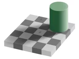
Edge Attneaves Cat 1954 2 Edges are caused by a variety of factors depth discontinuity surface color discontinuity illumination discontinuity surface normal discontinuity Origin of edges ID: 1031205
Download Presentation The PPT/PDF document "Edge Detection CSE 455 Linda Shapiro" is the property of its rightful owner. Permission is granted to download and print the materials on this web site for personal, non-commercial use only, and to display it on your personal computer provided you do not modify the materials and that you retain all copyright notices contained in the materials. By downloading content from our website, you accept the terms of this agreement.


1. Edge DetectionCSE 455Linda Shapiro
2. EdgeAttneave's Cat (1954) 2
3. Edges are caused by a variety of factors.depth discontinuitysurface color discontinuityillumination discontinuitysurface normal discontinuityOrigin of edges
4. Characterizing edgesAn edge is a place of rapid change in the image intensity functionimageintensity function(along horizontal scanline)first derivativeedges correspond toextrema of derivative4
5. The gradient of an image: The gradient points in the direction of most rapid change in intensityImage gradient5
6. The discrete gradientHow can we differentiate a digital image F[x,y]?Option 1: reconstruct a continuous image, then take gradientOption 2: take discrete derivative (“finite difference”)6
7. The gradient direction is given by: How does this relate to the direction of the edge?The edge strength is given by the gradient magnitudeSimple image gradientHow would you implement this as a filter?7perpendicularor varioussimplifications0 -1 1
8. Sobel operator-101-202-101-1-2-1000121Magnitude:Orientation:In practice, it is common to use:What’s the C/C++ function?Use atan2Who was Sobel?
9. Sobel operatorOriginalOrientationMagnitude
10. Effects of noiseConsider a single row or column of the imagePlotting intensity as a function of position gives a signalWhere is the edge?10
11. Effects of noiseDifference filters respond strongly to noiseImage noise results in pixels that look very different from their neighborsGenerally, the larger the noise the stronger the responseWhat can we do about it?Source: D. Forsyth11
12. Where is the edge? Solution: smooth firstLook for peaks in 12
13. Differentiation is convolution, and convolution is associative:This saves us one operation:Derivative theorem of convolutionfSource: S. SeitzHow can we find (local) maxima of a function?13We don’tdo that.
14. Remember:Derivative of Gaussian filterx-directiony-direction14
15. Laplacian of GaussianConsider Laplacian of GaussianoperatorWhere is the edge? Zero-crossings of bottom graph15
16. 2D edge detection filters is the Laplacian operator:Laplacian of GaussianGaussianderivative of Gaussian16
17. Edge detection by subtractionoriginal17
18. Edge detection by subtractionsmoothed (5x5 Gaussian)18
19. Edge detection by subtractionsmoothed – original(scaled by 4, offset +128)19
20. Using the LoG Function(Laplacian of Gaussian)The LoG function will beZero far away from the edgePositive on one sideNegative on the other sideZero just at the edgeIt has simple digital mask implementation(s)So it can be used as an edge operatorBUT, THERE’S SOMETHING BETTER20
21. Canny edge detectorThis is probably the most widely used edge detector in computer visionJ. Canny, A Computational Approach To Edge Detection, IEEE Trans. Pattern Analysis and Machine Intelligence, 8:679-714, 1986. Source: L. Fei-Fei21
22. The Canny edge detectororiginal image (Lena)22Note:I hate theLena images.
23. The Canny edge detectornorm of the gradient23
24. The Canny edge detectorthresholding24
25. Get Orientation at Each Pixeltheta = atan2(-gy, gx)25
26. The Canny edge detector26
27. The Canny edge detectorthinning(non-maximum suppression)27
28. Non-maximum suppressionCheck if pixel is local maximum along gradient directionPicture from Prem K Kalra28
29. Compute Gradients (DoG)X-Derivative of GaussianY-Derivative of GaussianGradient Magnitude29
30. Canny Edges30
31. Canny on Kidney 31
32. Canny CharacteristicsThe Canny operator gives single-pixel-wide images with good continuation between adjacent pixelsIt is the most widely used edge operator today; no one has done better since it came out in the late 80s. Many implementations are available.It is very sensitive to its parameters, which need to be adjusted for different application domains.32
33. Effect of (Gaussian kernel spread/size)Canny with Canny with original The choice of depends on desired behaviorlarge detects large scale edgessmall detects fine features33
34. An edge is not a line...How can we detect lines ?34
35. Finding lines in an imageOption 1:Search for the line at every possible position/orientationWhat is the cost of this operation?Option 2:Use a voting scheme: Hough transform 35
36. Connection between image (x,y) and Hough (m,b) spacesA line in the image corresponds to a point in Hough spaceTo go from image space to Hough space:given a set of points (x,y), find all (m,b) such that y = mx + bxymbm0b0image spaceHough spaceFinding lines in an image36
37. Hough transform algorithmTypically use a different parameterizationd is the perpendicular distance from the line to the origin is the angle of this perpendicular with the horizontal.37
38. Hough transform algorithmBasic Hough transform algorithmInitialize H[d, ]=0for each edge point I[x,y] in the image for = 0 to 180 H[d, ] += 1Find the value(s) of (d, ) where H[d, ] is maximumThe detected line in the image is given byWhat’s the running time (measured in # votes)? 38How big is the array H?Do we need to try all θ?dArray H
39. Example 0 0 0 100 100 0 0 0 100 100 0 0 0 100 100100 100 100 100 100100 100 100 100 100 - - 0 0 - - - 0 0 - 90 90 40 20 -90 90 90 40 - - - - - - - - 3 3 - - - 3 3 - 3 3 3 3 - 3 3 3 3 - - - - - -360 . 6 3 0 - - - - - - - - - - - - - - - - - - - - - 4 - 1 - 2 - 5 - - - - - - -0 10 20 30 40 …90360 . 6 3 0- - - - - - - - - - - - - - - - - - - - - * - * - * - * - - - - - - -(1,3)(1,4)(2,3)(2,4)(3,1)(3,2)(4,1)(4,2)(4,3)gray-tone imageDQTHETAQAccumulator HPTLISTdistance angle39
40. Chalmers University of Technology40
41. Chalmers University of Technology41
42. How do you extract the line segments from the accumulators?pick the bin of H with highest value Vwhile V > value_threshold { order the corresponding pointlist from PTLIST merge in high gradient neighbors within 10 degrees create line segment from final point list zero out that bin of H pick the bin of H with highest value V }42
43. Line segments from Hough Transform43
44. ExtensionsExtension 1: Use the image gradientsamefor each edge point I[x,y] in the image compute unique (d, ) based on image gradient at (x,y) H[d, ] += 1samesameWhat’s the running time measured in votes?Extension 2give more votes for stronger edgesExtension 3change the sampling of (d, ) to give more/less resolutionExtension 4The same procedure can be used with circles, squares, or any other shape, How?Extension 5; the Burns procedure. Uses only angle, two different quantifications, and connected components with votes for larger one.44
45. A Nice Hough VariantThe Burns Line Finder1. Compute gradient magnitude and direction at each pixel.2. For high gradient magnitude points, assign direction labels to two symbolic images for two different quantizations.3. Find connected components of each symbolic image.1234567812345678 Each pixel belongs to 2 components, one for each symbolic image. Each pixel votes for its longer component. Each component receives a count of pixels who voted for it. The components that receive majority support are selected.-22.5+22.504545
46. Example46Quantization 1 Quantization 2Quantization 1 leads to 2 yellow components and 2 green.Quantization 2 leads to 1 BIG red component.All the pixels on the line vote for their Quantization 2 component. It becomes the basis for the line.1234567812345678-22.5+22.50
47. Burns Example 147
48. Burns Example 248
49. Hough Transform for Finding CirclesEquations: r = r0 + d sin c = c0 - d cos r, c, d are parametersMain idea: The gradient vector at an edge pixel points to the center of the circle.*(r,c)d49
50. Why it worksFilled Circle: Outer points of circle have gradientdirection pointing to center.Circular Ring:Outer points gradient towards center.Inner points gradient away from center.The points in the away direction don’taccumulate in one bin!50
51. 51Procedure to Accumulate Circles Set accumulator array A to all zero. Set point list array PTLIST to all NIL. For each pixel (R,C) in the image { For each possible value of D { - compute gradient magnitude GMAG - if GMAG > gradient_threshold { . Compute THETA(R,C,D) . R0 := R - D*sin(THETA) . C0 := C + D*cos(THETA) . increment A(R0,C0,D) . update PTLIST(R0,C0,D) }}
52. 52
53. Finding lung nodules (Kimme & Ballard)53
54. FinaleEdge operators are based on estimating derivatives.While first derivatives show approximately where the edges are, zero crossings of second derivatives were shown to be better.Ignoring that entirely, Canny developed his own edge detector that everyone uses now.After finding good edges, we have to group them into lines, circles, curves, etc. to use further.The Hough transform for circles works well, but for lines the performance can be poor. The Burns operator or some tracking operators (old ORT pkg) work better.54