
siesta Alberto García After running siesta and compute the PDOS we can analyze the character of the different bands Which atoms contribute more to the bands at a particular ID: 659574
Download Presentation The PPT/PDF document "Javier Junquera How to plot fat bands ..." is the property of its rightful owner. Permission is granted to download and print the materials on this web site for personal, non-commercial use only, and to display it on your personal computer provided you do not modify the materials and that you retain all copyright notices contained in the materials. By downloading content from our website, you accept the terms of this agreement.


Slide1
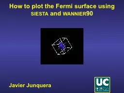
Javier Junquera
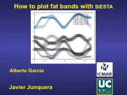
How to plot fat bands with siesta
Alberto
GarcíaSlide2
After running siesta
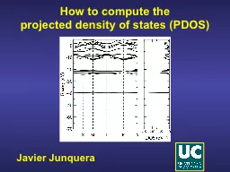
and compute the PDOS, we can analyze the character of the different bandsWhich atoms contribute more to
the bands at a particular energy windowSlide3
Fat bands: plot both
band eigenvalues and information about orbital projections on same foot Top of valence bands
: mostly O character
Bottom of conduction bands: mostly Ti characterWe can project on particular atomic orbitals within an atom to
further
define the
character.Slide4
A couple of utility programs must be compiled to run this exercise
$ cd <your_siesta_directory>/Util/COOP$ make OBJDIR=Obj$ cd <your_siesta_directory>/Util/Bands$ make OBJDIR=ObjReplace
Obj by the directory
where you have compiled siesta (the path should start at the same level than the Obj or
Src
directories)Slide5
New variables in siesta
to plot the fat bandsThese ranges can also be specified with
WFS.Energy.MaxWFS.Energy.MinSlide6
New variables in siesta
to plot the fat bandsThis will produce files with the extensionsSystemLabel.HSXSystemLabel.bands.WFSXSystemLabel.WFSX
The
unformatted WFSX files contain the information of the k-points for which wavefunctions coefficients are written, and the energies and coefficients
of each
wavefunction
which was specified in the input file. It
also
contains
information
on
the
atomic
species
and
the
orbitals
for
postprocessing
purposes
.
The
unformatted
H
SX file
contains
the
information
about
the
overlap
matrices as
well
as
other
data
required
to
generate
bands
and
density
of
statesSlide7
Prepare an input file required by the auxiliary utility code that produces the fat bands
System LabelName of the output file where
……the
eigenvalues and the projection weight for this orbital set will be storedWe need to compute the projected density
of states
for
the creation of fat bands plots
The
orbital sets are
included
as:
Atomic
symbol_shell
SystemLabel.mprSlide8
Run the utility code to fat bands
Output files
produced
Output of a successful runSlide9
Process the EIGFAT files produced in the previous run to generate files that can be read by a
ploterFor this, we will use the eigfat2plot files,
included in the Util/Bands
directoryProduce the file
to plot
the
band structureSlide10
Plot the band structure with gnuplotSlide11
Focusing on the top of the valence band and the bottom of the conduction bands
Clear hybridization of Ti t2g and O 2p orbitals
Small
contributions of the O 2p on the bottom of the conduction band
Small contributions
of the
Ti 3d on top of the valence band