/
On the occurrence of wave breaking Abstract Introduction Wave breaking criteria Kinematic On the occurrence of wave breaking Abstract Introduction Wave breaking criteria Kinematic

On the occurrence of wave breaking Abstract Introduction Wave breaking criteria Kinematic - PDF document

ellena-manuel
ellena-manuel . @ellena-manuel
Follow
533 views
Uploaded On 2014-12-19

On the occurrence of wave breaking Abstract Introduction Wave breaking criteria Kinematic - PPT Presentation

2 04 06 Nm Time UTC 123 4 m 123 4 Figure 2 Breaking scale 05 01 02 brk c 1 05 01 02 03 brk c 2 05 01 02 03 brk c 3 05 01 02 03 brk c 4 Figure 3 brPage 6br EZ EZ v 05 10 87226 10 87225 10 87224 10 87223 cc c m 87222 s Figure 4 Total breaking rate ZZ b ID: 26160

Time

Share:

Link:

Embed:

Download Presentation from below link

Download Pdf The PPT/PDF document "On the occurrence of wave breaking Abstr..." is the property of its rightful owner. Permission is granted to download and print the materials on this web site for personal, non-commercial use only, and to display it on your personal computer provided you do not modify the materials and that you retain all copyright notices contained in the materials. By downloading content from our website, you accept the terms of this agreement.


Presentation Transcript

124 GEMMRICH Geometric breaking criterion It would seem to be straightforward to monitor wave steepness. However, the steepness of individual waves cannot be defined uniquely in a broad band wave field. The challenge lies in defining an individual wave. Let us consider three different approaches to the analysis of a fixed point surface elevation time series (i) Zero-crossing analysis: A wave might be de-fined as the period between two successive in- =0, � 0, i.e. the period between two local wave troughs, and the wave height which is defined as the difference between the surface eleva-tions at the crest and the leading trough (Figure 1).The wave amplitude is a = . The linear disper-sion relation yields the wave number defines the local wave steepness. However, if shorter waves are riding on longer waves this method splits the underlying long wave and yields unrealisti-cally large steepness values, as it underestimates (Figure 1b). To rectify this bias, Banner et al. (2002) applied a riding wave removal scheme which progres-sively detects and removes riding waves through itera-tive processing starting with the highest frequency re-solved. The occurrence and characteristic dimensions of riding waves are retained in a file and a wave is then removed from the elevation series by replacing it with a cubic polynomial spliced to the underlying longer wave form. Subsequently, the association between breaking events and recorded waves is based on minimizing the relative lag between the time of the breaking event and the time of the nearest local crest, while also satisfying a local steepness threshold. (ii) Hilbert analysis: The Hilbert transform of a signal 1(')()'(') tPdtDue to a possible singularity at , the integral has to be taken as a Cauchy principal value P. The Hilbert transform defines the local amplitude 1/2()()locaXtHt, (2) loct , (3) tan()/() tXt. (Note, if ()cos() 4 6 8 10 1 2 2 1 0 1 2 Time [s] 4 6 8 10 1 2 3 2 1 0 1 2 3  . Surface elevation time series illustrating indi-vidual wave definition by zero-crossing analysis. are the height and period of the detected individual wave. a) No riding wave. b) A riding wave splits the underlying long wave. it follows ()sin() and () ). However, the classical Hilbert analysis is most meaningful for nar-row-banded signals. Broad-banded signals, like sur-face elevation records, have to be divided into a finite number of intrinsic mode functions (IMF), by way of empirical mode decomposition (EMD), before the Hilbert analysis can be applied (Huang et al., 1998). An IMF is defined as a function fulfilling the condi-tion that the number of zero-crossings and the num-ber of local maxima differ by not more than one. The IMFs are generated in an iterative way as the differ-ence between the signal and the mean of a spline fit-ting through all local maxima and a spline fitting through all local minima. This sifting process is re-peated until the IMF conditions are met. The so ob-tained IMF is subtracted from the time series and the iteration continues with the residual signal until only a monotonic signal remains. Typically, surface height records yield decomposition into (10) IMFs. Then, the surface elevation time series may be repre- OCCURRENCE OF WAVE BREAKING 125()()exp()tatit, (4) ()/tddt are amplitude, phase and frequency of the IMFs, respectively. The instanta-neous amplitude of the signal is ()()Atat (5) and the instantaneous frequency is , where cor-responds to the dominant IMF at time ()max((),1...)atatjN A defines steepness of the instantaneous dominant wavethat we chose the total amplitude A(t) rather than the amplitude of the dominant IMF . At a single point all IMFs contribute to the surface height but the domi-nant wavelength is not affected by high frequency IMFs. However, at the crest location of locally domi-nant waves the difference between A(t) and is not very significant. (iii) Wavelet analysis: The analysis seeks segments of the time series which resemble a short, predefined wavelet. By choosing a suitable form of the wavelet, small wave groups are detected and the associated wave steepness may be calculated. The wavelet transform of a is 1/2(,)()WpqpXtdt, (6) where the function is the wavelet. Particularly well suited for wave slope analysis is the Morlet wave- ()exp(/)exp(/)/2iKqpqp=−− (7) where the constant K determines the number of oscil-lation of the wavelet. In the case of the Morlet wavelet, the local peak, at a given , of the wavelet transform (,)Wpq represent the scale of the wave the location of the wave crest, is directly pro-portional to the average steepness of the group detected by the wavelet transform ()(,)akCWpq. The pro-portionality factor has to be determined from the wavelet analysis of simple known sinusoid test cases Scott et al., 2005). The dynamic wave breaking criterion is the most amenable to oceanic observations. In fact, the primary measurement of wave rider buoys is acceleration and only its double integration yields the surface elevation. Thus, in principle, wave riders may be used to detect wave breaking. Major limitations are the crest avoid-ance of the buoy and sensor tilt which results in a reduc-tion of the gravitational acceleration along the sensor axis and therefore an apparent upward acceleration. Also, there is uncertainty about the acceleration thresh-old associated with wave breaking. Some observations give /2 as expected (e.g. Snyder et al., 1983) but other observations show wave breaking at accelerations less than e.g. Holthujsen and Herbers, 1986). Indirect breaking criteria A fourth class of wave breaking definitions is based on the post-breaking signature, most commonly the visual signal of air entrainment (whitecapping) (e.g. Melville , 2002). Somewhat more objective meas-urements, but dependent on an unknown threshold, are sub-surface conductivity changes (Gemmrich and Farmer, 1999) or underwater sound (Ding and Farmer,1994). Microscale breakers do not entrain air but may be detected, with infrared imagers, as surface skin disruption et al.Wave breaking probability Traditionally, the frequency of wave breaking has been defined as the total number of breaking crests pass-ing a fixed point per unit time. Alternatively, the breaking probability per dominant wave is: brkPP , (8) is the dominant wave frequency. At first glance, the breaking frequency correlates with wind speed (more frequent breaking at increased wind speed) and to a somewhat lesser extend with wave age (reduc-tion in wave breaking as the wave age increases). How-ever, at best these correlations hold for individual storm events and different observations at similar wind speed or wave age report vastly different breaking probabili-ties. For a short review see Gemmrich and Farmer(1999) where the authors also report a significant posi-tive correlation between breaking probability and the energy input from the atmosphere into the wave field, normalized by the wind energy input into a developed It is well known even to the casual observer that wave breaking occurs at a wide range of scales. This breaking scale is of great importance to all physical processes as- OCCURRENCE OF WAVE BREAKING 127yields the apparent breaking wave speed as well as its . Smaller breaking waves are likely advected by the orbital motion of underlying larger . This Doppler shift is removed, based on the modified dispersion relation obsorb (16) , and the true wave propagation speed corresponding to the intrinsic frequency , is ob-tained. We base speed estimates on the average propa-gation speed within 0.3 s of detection and length esti-mates on the average object length calculated from all image frames. Thus, each whitecap is assigned one , one crest length and one propagation direc- . Note, this is different to the method reported by Melville and Matusov (2002) which is based on decom-posing the boundary of each whitecap into a number of elements each of a scale of approximately 0.5 m. Using PIV they estimated the length and the velocity relative to the whitecap centroid for each element. Elements with a positive, forward relative velocity are considered to be actively breaking. All actively breaking elements entered the statistics, with a single whitecap con-tributing to various different speeds. Wave field information utilized in this report is based on single point acoustic range finder data, kindly pro-vided by Dr. Jessup (APL, Seattle) Occurrence and scale of wave breaking Here we report on four data sets recorded under various wind forcing and wave field conditions (Figure 2). Data set 1 represents a growing sea, sets 2 and 3 nearly fully developed seas, and set 4 a growing sea in the presence of significant swell. 01/10 08/10 0 0.2 0.4 0.6 2]Time [UTC]1234 1 2 3 4 5 1234 Significant wave height (top panel) and wind during FAIRS. Numbers 1-4 indicate the timing of the data sets presented in this study. Wave breaking occurs over a wide range of scales (Figure 3). However, the breaking scales cover different ranges of the wave spectrum, depending on wave devel-opment. In the young sea case, phase speeds of breaking waves span from approximately 1/10 of the dominant phase speed ( with a wavelength corresponding to 1/100 of the dominant wavelength) up to the dominant waves. On the other end, in a fully developed sea we ob-served hardly any breaking at scales corresponding to phase speeds larger than about . As the wave age in-creases the distribution of breaking scales narrows sig-nificantly and the peak of the breaker phase speed distri-bution shifts from about 0.4 0.5 1 0 0.1 0.2 brk/cpP 1 0.5 1 0 0.1 0.2 0.3 brk/cpP 2 0.5 1 0 0.1 0.2 0.3 brk/cpP 3 0.5 1 0 0.1 0.2 0.3 brk/cpP 4 Figure 3. Distributions of the scale of breaking waves for four data sets indicated in Fig. 2; are the phase speeds of breaking waves and dominant waves, re-spectively. In terms of directional distribution we do not see any significant differences between the four data sets. The Gaussian distributions center around the mean wind di-rection and have a standard deviation of approximately Generally, the breaking crest length of individual events increases with wave scale. Therefore, the total breaking crest length per unit area and propagation speed, ), shows a slightly different behaviour than the break-ing occurrence rates given in Figure 3. For all four data segments, ) peaks at intermediate wave scales corre-c/c’ (1985) concept of a spectral equilibrium range assumes for intermediate wave scales a balance 128 GEMMRICH between energy input, non-linear energy transfer and energy dissipation. In this equilibrium range the wave height spectrum scales as . (17) Therefore, the form of the energy input ()()EgS (18) and the wave growth factor (/) 1982), (19) is some measure of the wind speed, translates into a dependence of the spectral wind energy input in c-space, . The equilibrium concept re-quires the same -dependence of the spectral dissipation and therefore, based on (13), it follows that 0.5 1 106 105 104 103 2s] Figure 4. Breaking crest length as function of normalized crest propagation speed p , i.e. the normalized phase speed of breaking waves. The symbols ,*,+) correspond to data sets (1,2,3,4), respectively. At scales larger than the peak of the observed ) indeed falls off approximately as consistent with the equilibrium range concept. (Although this does not show clearly in Figure 4 it is seen in a graph as will be described in a forthcoming paper). However, according to (13) the low at small scales imply reduced dissipation, and thus the equilibrium concept requires reduced energy input and/or increased non-linear transport to larger wave scales com-pared to the current formulation of spectral wave models. It should be noted that the inferences made about the slope of ) are based on the assumption that the pro-portionality factor in (13) is scale independent, as found in the somewhat unrelated hydrofoil experiment by (1981). Moreover, the value of is very uncer-tain with reported values applicable to the ocean ranging from Phillips et al., 2001) to , 2002) and assumed to be scale inde-The overall breaking rate R , given by (12), is equiva-lent to the fractional surface area turnover rate, and thus an important quantity for air-sea exchange processes. It also provides insight to what conditions are favourable to wave breaking. Banner et al. (2002) found the breaking rate at specific scales to depend on some measure of the mean steepness. Here we explore possible correlations between the total breaking rate and wave steepness. In this context it is interesting to note that in wave tank experiments the wave groupiness, believed to play an important role in the generation of rogue waves, also de-termines the limiting steepness max of these extreme Wu and Yao, 2004). Assuming that larger wave amplitudes, i.e. steeper waves, are prevented due to wave breaking implies that the steepness threshold of the geo-metric wave breaking criterion is equal to maxWu and Yao (2004) report a very strong inverse de-pendence of the maximum attainable wave steepness max on the non-dimensional wave group bandwidth 11 (20) 3/21/2mSd is the i moment of the power spectrum S(Longuet-Higgins, 1984). For long groups ( , i.e. narrow peaked spectrum) maxclose to the Stokes limit /7, whereas for (shorter groups, broader spectrum) the authors found a sharply reduced value max0.2If wave breaking is the limiting process, one would ex-pect that in cases of small max wave breaking is more frequent than in cases with a larger limiting steep-ness, yielding a positive correlation between wave breaking and bandwidth. No well defined relation be-tween breaking rate and bandwidth emerges from our data, which might, however, partially be due to the lim- OCCURRENCE OF WAVE BREAKING 129ited range of bandwidth in our observations (Figure 5a). It is very likely that processes associated with the direc-tional wave field (e.g. directional focusing) are impor-tant for wave breaking and the excellent correlation be- observed in the controlled 2-dimensional wave tank environment might also not be as strong under open ocean conditions. The fact that the limiting steepness of extreme waves varies widely also suggests that the critical wave steepness that will lead to wave breaking does not have a fixed value. Nevertheless, one expects a wave field with a significant fraction of ‘steep’ waves to exhibit more breaking than a wave field with fewer ‘steep’ waves. To test this assumption we calculate the steepness for each individual wave crest and determine the fraction of wave crests with steepness above a given threshold. The breaking rate increases approximately linearly with the fraction of steep waves (Figure 5b). It turns out that this scaling is not very sensitive to the threshold steep-ness values if chosen in the range 0.3 – 0.45, though ab- 0.15 0.2 0.25 0.3 0.35 0. 4 0 20 40 60 80 100 120 R [h1] 0.005 0.01 0.015 0.0 2 0 20 40 60 80 100 120 1] Figure 5. Breaking rate R (equation 12) versus nondimen-sional bandwidth (equation 20) (top) and fraction of wave crests with wave steepness larger than /7 (bottom). Wave breaking criteria based on geometric, kinematic or dynamic properties of individual waves are not easily applicable to oceanic observations, mainly due to uncer-tainties in identifying individual waves and unknown threshold values. Most accessible is the post-breaking criterion of whitecap generation. (1985) equilib-rium range theory includes a statistical description of wave breaking, its kinematics and dynamics. The re-quired key quantity cdc is the length of breaking crests per unit area propagating with speeds in the range (,)ccdc , may be extracted from video imagery of the sea surface. peaks at intermediate wave scales and for larger scale it is approximately pro-portional to c which is consistent with the current form of spectral wave models. However, the steep decline of at small scales implies reduced energy input and/or more rapid non-linear transfer in order to satisfy the equilibrium assumption. However, the uncertainty in the proportionality factor length to energy dissipation, further complicates this is-sue. Independent co-located measurements of energy are required to determine whether the proportionality factor is in-deed independent of In a young wave field, breaking that generates white-caps occurs at a wide range of scales corresponding to breaking wave phase speeds from about 0.1 – 1.0 . The most frequent breakers occur at scales corresponding to p. In developed seas the distribution of breaker speeds narrows, with almost all breaking wave speeds , and the peak of the distribution shifts to 0.2 As wave breaking is the main limiting factor of wave growth, the breaker scale distribution is also expected to impact processes like rogue wave generation. Breaking of waves close to the dominant wave scales would severely limit the generation of rogue waves. Thus, the lack of breaking of large scale waves in older seas implies a much greater likelihood of rogue wave occurrence in developed seas than in young seas. In wave tanks the wave-group bandwidth seems to be a very good indicator of limiting extreme wave steepness, with reduced attainable steepness as the wave spectral bandwidth increases (Wu and Yao, 2004). It is not en-tirely clear whether the limiting extreme wave steepness is equivalent to the critical steepness that leads to break-ing. If this was the case, the breaking rate would be a wave spectral bandwidth, which is not supported in our open ocean data set. Since