Drill: Find the differential of each equation. - PowerPoint Presentation

Slide1

Drill: Find the differential of each equation.

y = exy = e4xy = ex^2y = sec x

dy

= e

x

dx

dy

= 4e

4x

dx

dy

= 2xe

x^2

dx

dy

=

tanxsecx

dx

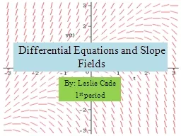
Slide2

Slope Fields and Euler’s Method

Lesson 6.1

Slide3

Objectives

Students will be able to:construct antiderivatives using the Fundamental Theorem of Calculus.solve initial value problems in the formconstruct slope fields using technology and interpret slope fields as visualizations of different equations.use Euler’s Method for graphing a solution to an initial value problem.

Slide4

Differential EquationAn equation involving a derivative is called a differential equation

. The order of a differential equation is the order of the highest derivative involved in the equation.

Slide5

Example

Solving a Differential EquationFind all functions y that satisfy Solution: the anti-derivative of dy/dx:This is called a GENERAL solution.We cannot find a UNIQUE solution unless we are given further information.

Slide6

If the general solution to the first order differential equation is continuous, the only information needed is the value of the function at a single point, called an INITIAL CONDITION.A differential equation with an initial condition is called an INITIAL VALUE PROBLEM.

It has a unique solution, called the PARTICULAR SOLUTION to the differential equation.

Slide7

Example

Solving a Differential EquationFind all the functions y that satisfy

Slide8

Example

Solving an Initial Value ProblemFind the particular solution to the equationwhose graph passes through the point (0, 1).

Slide9

Example

Solving an Initial Value ProblemFind the particular solution to the equationand y

= 60 when

x

= 4.

Slide10

Example

Handling DiscontinuityFind the particular solution to the equation dy/dx = 2x – sec2x whose graph passes through the point (0, 3)The general solution is y = x2 – tanx + CApplying the initial condition: 3 = 02 – tan0 + C; 3 = CTherefore, the particular solution is y = x

2

–

tanx

+ 3

However, since because

tanx

is does have discontinuities, you need to add the domain stipulation of –

π

/2 < x<

π

/2

Slide11

Example

Using the Fundamental Theorem Find the solution to the differential equation f’(x) = e-x^2 for which f(7) = 3Rather than determining the anti-derivative, you can let the solution in integral form:We know that ifThen ANDf’(x) = e-x^2

This is our solution!

Note: If you are ABLE to determine the anti-derivative, you should do so!

Slide12

Drill: Find the constant Cy = 3x

2 + 4x + C and y = 2 when x = 1y = 2sinx – 3cosx + C and y = 4 when x = 02 = 3(1)2 + 4(1) + C2=3+4+C2 = 7 + C-5 = C4 = 2sin(0) – 3cos(0) + C4 = 0 – 3 + C4 = -3 + C7 = C

Slide13

Graphing a General SolutionGraph the family of functions that solve the differential equation dy

/dx = cos xAny function of the form y = sinx + C solves the differential equation.First graph y = sin x, and then repeat the graph by shifting vertically up and down.

Note: you can also use the calc by putting values of ‘C’ in to L

1

and then graphing y

1

=

sinx

+ L

1

Slide14

Slope Fieldsa slope field (or

direction field) is a graphical representation of the solutions of a first-order differential equation. It is achieved without solving the differential equation analytically. The representation may be used to qualitatively visualize solutions, or to numerically approximate them.Remember also, that the derivative of a function gives its slope.Also remember that we use the notation dy/dx to represent derivative; therefore, dy/

dx

= slope.

Slide15

A Summary of Making Slope FieldsPut the differential equation in the form dy

/dx = g(x,y)Decide upon what rectangular region of the plane you want to make the pictureImpose a grid on this regionCalculate the value of the slope, g(x,y), at each grid point, (x,y)Sketch a picture in which at each grid point there is a short line segment having the corresponding slope

Slide16

Example: Constructing a Slope FieldConstruct a slope field for the differential equation dy

/dx = cos xWe know that that slope at any point (0, y) will be cos (0) = 1, so we can start be drawing tiny segments with slope 1 at several points along the y-axis.Slope is also 1 at 2π, - 2πWhen would the slope by -1?At π, - π

When is the slope 0?

At

π

/2, -

π

/2

At 3

π

/2, -

3

π

/2

Slide17

Solutionx: [-5π/2, 5π/2]; y: [-4, 4]

Slide18

Example

Matching Slope Fields with Differential Equations Use slope analysis to match the differential equation with the given slope fields. Note: each block is .5 units.

Slide19

Example

Matching Slope Fields with Differential Equations Use slope analysis to match the differential equation with the given slope fields. Note: each block is .5 units

Slide20

Example

Matching Slope Fields with Differential Equations Use slope analysis to match the differential equation with the given slope fields. Note: each block is .5 units

Slide21

Example

Matching Slope Fields with Differential Equations Use slope analysis to match the differential equation with the given slope fields. Note: each block is .5 units

Slide22

Example

Matching Slope Fields with Differential Equations Use slope analysis to match the differential equation with the given slope fields. Note: each block is .5 units

Slide23

Example

Matching Slope Fields with Differential Equations Use slope analysis to match the differential equation with the given slope fields. Note: each block is .5 units

Slide24

Constructing a Slope Field for a Nonexact Differential Equation

Construct a slope field for the differential equation dy/dx = x + y and sketch a graph of the particular solution that passes through (2, 0).You can make tables in order to graph slopes: (some examples) x + y = 0 x + y = -1 x + y = 1The particular solution can be found by drawing a smooth curve through the point (2, 0) that follows the slopes in the slope field.

x

y

-2

2

-1

1

0

0

1

-1

2

-2

x

y

-2

1

-1

0

0

-1

1

-2

2

-3

x

y

-2

3

-1

2

0

1

1

0

2

-1

Slide25

Solution http://www.math.rutgers.edu/~sontag/JODE/JOdeApplet.html

Slide26

DrillFind a solution that satisfies y(1) = 2 when

First, determine the anti-derivative.

Slide27

Euler’s MethodBegin at the point (x, y) specified by the initial condition. This point will be on the graph, as required.

Use the differential equation to find the slope dy/dx at the point.Increase x by a small amount of Δx. Increase y by a small amount of Δy, where Δy = (dy/dx) Δx. This defines a new point (x + Δx, y + Δy) that lies along the linearization.Using this new point, return to step 2. Repeating the process constructs the graph to the right of the initial point.

To construct the graph moving to the left from the initial

point,r

epeat

the process using negative values for

Δ

x.

Slide28

Example

Applying Euler’s Method Let f be the function that satisfies the initial value

problem and

f

(0) = 1. Use Euler’s

Method and increments of

Δ

x

= 0.2 to approximate

f

(1).

Slide29

Example

Applying Euler’s Method

Slide30

Example

Applying Euler’s Method Let f be the function that satisfies the initial value

problem and if y = 3 when x = 2, use

Euler’s Method with five equal steps to approximate y when x = 1.5.

Δ

x = (1.5 – 2)/5 = -.1

(Note,

Δ

x is negative when you are going backwards.

Slide31

Example

Applying Euler’s Method

Slide32

Homework

Day #1:Page 327: 1-19: oddDay #2: Page 327/8: 21-39: oddDay #3: page 328: 41-48