Energy consumption is increasing day by day with increasing population and soaring economies. - PowerPoint Presentation

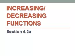
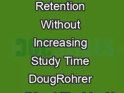
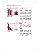
1. Energy consumption is increasing day by day with increasing population and soaring economies. The necessity for predicting and forecasting energy needs is more now than ever before. Energy forecasts play a vital role in energy optimization which is very important in balancing the energy supply and demand.The main objective of this poster is to use JMP Pro 11 to predict monthly energy consumption of individual household unit or business unit in United States of America based on the unit's historical consumption levels. The main steps involved in doing this forecast are data preparation, consumption pattern identification , seasonality factor analysis in time series data and estimation of the effect of external factors like the economic meltdown on energy consumption. Various models are built using JMP time series analysis and the best model is selected by assessing its performance on the validation data.The dataset gathered from EIA website has monthly energy consumption records of individual household units or business units in United States of America from the year 2000 to 2014. The last 24 months of data has been used as a hold out sample to check the model performance in predicting the consumption levels. The dataset aggregated to fit for time series analysis has a time id, total energy consumption r of the individual household or business unit in Trillion BTU Units recorded in one month. Trend and Seasonality Analysis: Trend represents a general systematic linear or quadratic component that changes over time and does not repeat within the time range captured in the data whereas Seasonality is a trend that repeats itself systematically over time. There is strong seasonality pattern in our data as the energy consumption varies during the year with January having the highest consumption. Auto correlation and partial autocorrelation graphs are examined for the seasonal patterns.Actual Energy Consumption and seasonality Pattern:Energy Consumption Forecast Using JMP® Pro 11 Time Series AnalysisPradeep Kalakota, Graduate Student, Oklahoma State UniversitySrinivas Reddy Busi Reddy, Graduate Student, Oklahoma State University Graph with actual consumption vs month Graph with consumption over different monthsDifferencing: We have used differencing of 1 to remove seasonal pattern to discover any unusual trend other than seasonality.Auto- Correlation and Partial Auto-correlation plots (before & after):Fig: Auto correlation and partial auto-correlation graphs before and after differencingAfter the initial data analysis the next process taken up was  the identification process for parameter estimates (auto regressive parameter, moving average parameter and differencing parameter) of the model. Major tools used in the identification phase are plots of the series, correlograms of auto correlation (ACF), and partial autocorrelation (PACF). A transfer function model has been built to analyze the effects of other input variables on energy consumption. It revealed that the years 2001, 2008 and 2009 had low energy consumption levels. This might be because of the economic meltdowns in those years. In model building stage, seasonal exponential smoothing model , winter’s additive model and ARIMA models are used to forecast the energy consumption. Then we have used the model comparison feature of JMP to compare the AIC and MAPE values of the models to find the best suited method to forecast. A transfer function model with a input series of effects of recession during this period is considered for comparison. From these results, there is a substantial affect of recession which shows that the consumption has actually reduced during these periods. Energy Consumption Forecast Using JMP® Pro 11 Time Series AnalysisPradeep Kalakota, Graduate Student, Oklahoma State UniversitySrinivas Reddy Busi Reddy, Graduate Student, Oklahoma State UniversityAbstractData PreparationInitial AnalysisModelsModel Comparison

2. Energy Consumption Forecast Using JMP® Pro 11 Time Series AnalysisPradeep Kalakota, Graduate Student, Oklahoma State UniversitySrinivas Reddy Busi Reddy, Graduate Student, Oklahoma State University Energy Consumption Forecast Using JMP® Pro 11 Time Series AnalysisPradeep Kalakota, Graduate Student, Oklahoma State UniversitySrinivas Reddy Busi Reddy, Graduate Student, Oklahoma State UniversityModel Fit Statistics and Results:Transfer Function Model StatisticsAppendixFrom the above Fit Statistics, based on MAPE value, Transfer function model is performing better and has the better forecast resultsFig: ForecastFig: Pre-whiteningConclusionThe training dataset contains 144 observations with monthly data points from 2000 to 2011. The 24 data points for the years 2012 and 2013 are held for the evaluation.Initial findings are the energy consumption in the months of January and February is the highest There is a drop in energy consumption during the effects of recession i.e. 2001, 2008, and 2009.Pre-whitening for transfer function model include removing the noise caused by seasonality and the input variable. The R-square value is 0.64 and the MAPE value is 1.44 which is the lowest among the models.Using JMP Pro 11's Save predicted values option, forecast results have been saved for each model and the functions concatenate and split have been used to build a table with all the forecast results.Transfer Function is the best model. We can forecast the energy consumption for 12 months with high accuracy and help in identifying supply and demand for energy.Forecast values of different models and comparison with actual valuesReferenceshttp://jmp.com/support/help/index.shtml/ https://statsoft.com/textbook/time-series-analysis/ http://www.jmp.com/about/events/summit2013/resources/Poster14_Reddy_Rayabaram.pdf http://www.eia.gov/totalenergy/ AcknowledgementWe thank Dr. Goutam Chakraborty, Founder of SAS and OSU Data Mining and Business Analytics Program at Oklahoma State University, for his continuous guidance and support throughout the project.