Estimating The Cyclically Adjusted Budget Balance For - PDF document

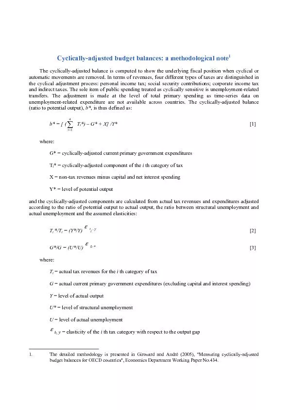
Estimating The Cyclically Adjusted Budget Balance For The Romanian Economy Romanian Journal of Economic Forecasting … 2/2010 79 STIMATINGTHECYCLICALLYADJUSTEDBHERCONOMY This paper provides estimates for the structural fiscal balance for the Romanian economy over the period 1998-2008. The calculation of the structural fiscal balance is useful, since it provides a clear picture of the fiscal stance of the economy and it is essential in the context of a medium term fiscal framework. In order to ensure the robustness of the estimation, we employed two methodologies for the computation of the elasticities of various categories of government revenues and expenditures with respect to the output gap. The two approaches issued similar results, the overall ave-rage budget sensitivity being equal to 0.285 and 0.290, respectively. The amplitude of the cyclical budget balance is around 1% of GDP. After constant improvement, the structural balance worsened in 2008, due mainly to the current crisis. Keywords: fiscal policy, structural fiscal balance, cyclical budget balance, business Government revenues and expenditures are affected by the cyclical position of the economy, due to the effect of automatic stabilizers. Several components of Financial Support provided by PN II PCE Grant 1863/2009 entitled Modeling the Influence of the Trinomial Uncertainty-Volatility-Risk on the Dynamics of Complex Financial-Economic SystemsŽ and by SPOS Grant 1/2009 entitled Romanian Medium Term Fiscal FrameworkŽ. DOFIN, Academy of Economic Studies, Bucharest; Center for Advanced Research in Finance and Banking (CARFIB); Centrul de Analiz Economico-Financiar(CAPEF); email: maltar@ase.ro Institute of Economic ForecastingRomanian Journal of Economic Forecasting … 2/201080 government budget are influenced by the macroeconomic stance in ways that operate to smooth the business cycle, acting as automatic stabilizers. For example, in a recession fewer taxes are collected, which operates to support private incomes and dampens the adverse movements in aggregate demand. Conversely, during a boom more taxes are collected, counteracting the expansion in aggregate demand. This stabilizing property is stronger if the tax system is more progressive. Another automatic fiscal stabilizer is the unemployment benefit system: in a recession the growing payment of unemployment benefits supports demand and the other way around occursin an upswing. If governments allow automatic an fiscal stabilizer to work fully in a recession but do to resist the temptation to spend cyclical revenue increases during an upswing, the stabilizers may lead to a bias toward weak underlying budget positions. The structural or cyclically adjusted budgetary balance is defined as the fiscal balance that would arise provided that output was at its potential level and, therefore, not reflecting the cyclical aspects in economic activity. Hagemann (1999) defines the structural fiscal balance as the residual balance after removing the balance of the estimated budgetary consequences of the business cycle. Therefore, the calculation of the structural fiscal balance is useful, as it provides a clearer picture of the underlying fiscal situation by subtracting from the impact of the business cycle. As a result, it can be used to guide fiscal policy analysis. One approach to examine the impact of discretionary fiscal policy over the cycle is to link the fiscal policy stance, generally measured as the change in the structural fiscal balance, to the cyclical conditions measured by the output gap. Econometric investigation covering the period from the mid-1990s to 2006 shows that the fiscal policy has been, on average, pro-The importance of assessing the structural fiscal balance has increased after Romania entered the European Union. The structural fiscal balance does play a key role in the European Union surveillance procedures, especially in the Stability and Growth Pact. Although the condition of the Pact concerning the ratio of government deficit to GDP refers to the actual rather than the structural deficit, the cyclically adjusted budget balance is employed within the SGP framework to measure the stance of fiscal policy. Also, the structural balance is used by the European Commission in assessing whether the prevailing fiscal situation in individual countries is sufficient to comply with the requirements of the Stability and Growth Pact, whether it is strong enough to provide for a safety margin that the actual budget deficit does not exceed the threshold of 3% of GDP during a recession. On the other hand, the Euro Area and the ERM II member states need to specify a country-specific medium-term budgetary objective that should range between -1% of GDP and in balance or surplusŽ, measured in cyclically adjusted terms, net of one-off effects and temporary Although several methodologies have been proposed (Giorno 1999; van der Noord, 2000; Bouthevillain et al., 2001; Congressional Budget Office, 2004; Girouard and Andre, 2005), there is no generally accepted method of quantifying the part of the current budgetary balance that reflects short-term transitory influences caused by cyclical factors and the part due to structural measures taken by fiscal authorities. Generally, the measurement of the cyclically adjusted budget balance proceeds in three steps. The first step involves the estimation of the potential Institute of Economic ForecastingRomanian Journal of Economic Forecasting … 2/201082 fixed elasticities hypothesized in the OECD and European Commission methodologies The rest of the paper is organized in three sections. In the second and third sections we estimate the structural fiscal balance for the Romanian economy using quarterly Quarterly Data In this section, we will employ quarterly data for the period 1998:Q1-2008:Q4. In order to estimate tax and expenditure elasticities, we will apply a methodology similar to that employed by the OECD and by the European Commission (Giorno et alden Noord, 2000). This approach involves the estimation of elasticities with respect to output for the various government revenue and expenditure categories. These elasticities, together with the estimated output gap, are then used to calculate the structural (i.e., not affected by cyclical conditions) tax revenues and expenditures. Every elasticity is decomposed in a number of components that can be estimated using the available data and specific econometric techniques. The OECD methodology computes for every government revenue and expenditure category a single elasticity for the whole period. Therefore, the estimated elasticities may be expected to reflect, at best, the average cyclical responsiveness of these revenue and expenditure items over a sample period. Actual quarter-to-quarter behavior may be more erratic as specific tax bases may react non-typically over the cycle. In this study, cyclically adjusted budget balance (CAB) is obtained by subtracting the cyclical cyclical component of each revenue or expenditure category ( ) is computed We will describe next the techniques employed to compute each category of tax elasticity and expenditures elasticity, as well as the estimated cyclical component for In order to compute the personal income tax elasticity, this elasticity is decomposed wLLwLPITwwLPITLYYLTYYLLPITPITYYPITPIT1consisting of several auxiliary elasticities: Institute of Economic ForecastingRomanian Journal of Economic Forecasting … 2/201084 where the stationary condition requires that 121 .The trend component is modeled as a random walk with drift: ttttzTT1 and the drift term itself is allowed to follow a random walk ttta1 where: The equations described above are estimated on quarterly data over the period 1998:Q1 to 2008:Q4 using the Maximum Likelihood Estimator of a bivariate Kalman Actual unemployment and NAIRU 1998Q11999Q12000Q12001Q12002Q12003Q12004Q12005Q12006Q12007Q12008Q1 unemployment rate, seasonally adjusted NAIRUNIS, authors calculations. The structural unemployment had a clear descending trend over the analyzed period. In Romania there are two series for the unemployment rate, reflecting different methodologies: the ILO (International Labor Office) unemployment rate, and the registered unemployment rate. Since in this paper the NAIRU is mainly used to compute the elasticity of the current expenditure, the registered unemployment rate was employed, because it reflects the actual number of people entitled to receive 2.1.2 The Output Elasticity of Employment The output elasticity of employment can be computed as the estimate of the *10*loglogYYaaLL Institute of Economic ForecastingRomanian Journal of Economic Forecasting … 2/201086 Figure 2The estimated income distribution in 2006 35060085011001350160018502100235026002850 Authors calculations. iiiiiiiiwPITdwdPITe - the wage income elasticity of income taxes; i - the weight of earnings-level i in total earnings according to the first- iidwdPIT - the marginal income tax rate at point i on the income distribution; - the average income tax rate at point i on the income distribution. In the Romanian case, the wage elasticity of the personal income tax varied between 1.57 and 2.09. After the flat rate regime was introduced, it was a significant reduction in the wage income elasticity, although it remained above 1, due to the existence of 2.1.5 The Cyclical Component of Personal Tax Income Revenues The estimates of the Personal Income Tax output elasticity for the period 1998:Q1-2008:Q4 are presented in Table A.2 in Appendix. The estimated average elasticity RON Institute of Economic ForecastingRomanian Journal of Economic Forecasting … 2/201088 the contribution rate is flat and there are no deductions, the wage elasticity of social security contributions is constant and equal to 1 for the entire 1998-2006 period. The estimates of the Social Security Contribution output elasticity for the period 1998:Q1-2008:Q4 are presented in Table A.2 in the Appendix. The estimated average elasticity over the entire sample is 0.751. The OECD cross-country average estimate is 0.81 with a standard deviation of 0.22 (van den Noord, 2000).The Social Security Contribution cyclical component 1998Q11999Q12000Q12001Q12002Q12003Q12004Q12005Q12006Q12007Q12008Q1% of actual level SSC cyclical componentAuthors calculations. Figure 4 depicts the cyclical component of social security contributions. In the analyzed period the amplitude of this cyclical component was around 4% of the actual level, the social security contributions being the least sensitive revenue component In the OECD methodology it is assumed that Corporate Income Tax elasticity is equal to the elasticity of the tax base (Corporate Income) with respect to output. The elasticity is decomposed into the profit share of national income, the output elasticity of employment (already estimated above) and the employment elasticity of wages The estimates of the Corporate Income Tax output elasticity for the period 1998:Q1-2008:Q4 are presented in Table A2 in the Appendix. The estimated average elasticity over the entire sample is 1.205. The OECD cross-country average estimate is 1.26 Figure 5 depicts the cyclical component of corporate income taxes. In the analyzed period, the amplitude of this cyclical component was around 6% of the actual level, the corporate income taxes being the most sensitive revenue component with respect to Institute of Economic ForecastingRomanian Journal of Economic Forecasting … 2/201090 The estimates of the Indirect Taxes output elasticity for the period 1998:Q1-2008:Q4 are presented in Table A.2 in the Appendix. The estimated average elasticity over the entire sample is 0.97. The OECD cross-country average estimate is 0.89 with a Figure 6 depicts the cyclical component of indirect taxes. In the analyzed period, the amplitude of this cyclical component was around 5% of the actual level.The methodology assumes that the current primary expenditure fluctuates in proportion to the unemployment-related expenditure and that unemployment-related expenditure is strictly proportional to unemployment. The elasticity is decomposed into the output elasticity of employment (already estimated above); the employment elasticity of the labor force; the is the current primary expenditure, is the unemployment, For the computation of the short-run employment elasticity of the labor force, the is the labor supply, and are actual and potential employment. The The Current Primary Expenditure Cyclical Component -0.6-0.5-0.4-0.3-0.2-0.10.10.20.30.40.50.60.71998Q11999Q12000Q12001Q12002Q12003Q12004Q12005Q12006Q12007Q12008Q1% of actual level CPE cyclical t Source: Authors calculations. Institute of Economic ForecastingRomanian Journal of Economic Forecasting … 2/201092 The Dynamics of the Structural Budget Balance 19981999200020012002200320042005200620072008% of GDP actual balance cyclical balance structural balanceSource: Authors calculations. The estimated cyclical components of the budget balance are surrounded by significant margins of uncertainty. Therefore, it is essential to check the robustness of these estimates using various methodologies. In this section, we will compute the following the methodology outlined in Girouard and Andre (2005), with the main difference consisting in the fact that in this paper the elasticity of various budget items is not fixed but allowed to vary on a year-to-year basis.Girouard and Andre (2005) updated the OECD methodology by introducing several innovations to account better for the lags between taxes and the stance of the business cycle and to ensure greater cross-country consistency in the estimates of the various budget categories elasticities, as well as to improve the statistical properties of the coefficients of the regressions linking the tax bases to the output gap. According to this methodology, every elasticity is separated into two components, namely an elasticity of tax incomes with respect to the relevant tax base, and an The elasticity of the tax income with respect to the tax base is determined by the in the case of the Personal Income Tax, it is given by the wage elasticity of the in the case of the Social Security Contribution, it is constant and equal to 1 Institute of Economic ForecastingRomanian Journal of Economic Forecasting … 2/201094 Actual Balance Cyclical Balance Structural Balance (% of GDP) (% of GDP) (% of GDP) 2004 -1.18 0.36 -1.54 2005 -0.79 -0.19 -0.60 2006 -1.64 0.34 -1.98 2007 -2.50 0.50 -3.00 2008 -5.40 1.00 -6.40 Source: Authors calculations. We obtained results almost identical to those in the previous section. The structural balance varied between -0.60% and -6.40% of the GDP. After a period of constant improvement in the structural fiscal stance, with a descending trend of the structural balance, the last period was characterized by a significant increase in the cyclically adjusted deficit. It will be quite a challenge to reach the medium term objective of a structural fiscal balance of -1.93% of the GDP for 2011 and -0.9% for 2012 as stated in the Convergence Program (Ministry of Public Finance, 2009).Figure 9 depicts the dynamics of the cyclically adjusted budget balance for the The Dynamics of the Structural Budget Balance 19981999200020012002200320042005200620072008% of GDP actual balance cyclical balance structural balanceSource:Authors calculations. The amplitude of the cyclical budget balance is around 1% of GDP, with a shape In this paper we estimated for the Romanian economy the structural fiscal balance in Institute of Economic ForecastingRomanian Journal of Economic Forecasting … 2/201096 Langedijk, S. and Larch M. (2007), Testing the EU fiscal surveillance: How sensitive is it to variations in output gap estimates?Ž, European Economy - Economic Papersvan der Noord, P., (2000), The Size and Role of Automatic Fiscal Stabilizers in the OECD Economics Department Working PaperWolswijk, G. (2007), Short and long-run tax elasticities. The case of the NetherlandsŽ, ***, Congressional Budget Office, (2004), ***, European Commission (2006), Public finances in EMU … 2006Ž, Economy***, European Commission (2007), Public finances in EMU … 2007Ž, Economy***, European Commission (2008), Public finances in EMU … 2008Ž, EconomyConvergence Programme 2008-2011 Institute of Economic ForecastingRomanian Journal of Economic Forecasting … 2/201098 1 2 3 4 5 6 7 2001Q1 1.096 0.751 1.205 0.970 -0.075 0.324 2001Q2 1.096 0.751 1.205 0.970 -0.072 0.290 2001Q3 1.096 0.751 1.205 0.970 -0.077 0.242 2001Q4 1.096 0.751 1.205 0.970 -0.090 0.241 2002Q1 1.158 0.751 1.198 0.970 -0.086 0.332 2002Q2 1.158 0.751 1.198 0.970 -0.084 0.282 2002Q3 1.158 0.751 1.198 0.970 -0.086 0.248 2002Q4 1.158 0.751 1.198 0.970 -0.077 0.240 2003Q1 1.120 0.751 1.204 0.970 -0.095 0.326 2003Q2 1.120 0.751 1.204 0.970 -0.096 0.285 2003Q3 1.120 0.751 1.204 0.970 -0.094 0.250 2003Q4 1.120 0.751 1.204 0.970 -0.092 0.240 2004Q1 1.106 0.751 1.212 0.970 -0.100 0.351 2004Q2 1.106 0.751 1.212 0.970 -0.099 0.291 2004Q3 1.106 0.751 1.212 0.970 -0.093 0.245 2004Q4 1.106 0.751 1.212 0.970 -0.115 0.235 2005Q1 1.004 0.751 1.196 0.970 -0.118 0.341 2005Q2 1.004 0.751 1.196 0.970 -0.121 0.300 2005Q3 1.004 0.751 1.196 0.970 -0.124 0.246 2005Q4 1.004 0.751 1.196 0.970 -0.128 0.245 2006Q1 0.965 0.751 1.200 0.970 -0.105 0.342 2006Q2 0.965 0.751 1.200 0.970 -0.108 0.293 2006Q3 0.965 0.751 1.200 0.970 -0.111 0.255 2006Q4 0.965 0.751 1.200 0.970 -0.113 0.250 2007Q1 0.965 0.751 1.208 0.970 -0.086 0.301 2007Q2 0.965 0.751 1.208 0.970 -0.088 0.286 2007Q3 0.965 0.751 1.208 0.970 -0.089 0.260 2007Q4 0.965 0.751 1.208 0.970 -0.091 0.245 2008Q1 0.965 0.751 1.201 0.970 -0.082 0.353 2008Q2 0.965 0.751 1.201 0.970 -0.083 0.302 2008Q3 0.965 0.751 1.201 0.970 -0.084 0.255 2008Q4 0.965 0.751 1.201 0.970 -0.086 0.227 Average 1.034 0.751 1.205 0.970 -0.102 0.285 Source: Authors calculations.