
Many applications of statistical analysis involves a continuous variable as dependent variable DV but both continuous and categorical variables as independent variables IV Relationship between DV and continuous IVs is linear and the slope remains the same in different groups ANCOVA ID: 653960
Download Presentation The PPT/PDF document "Xuhua Xia Fitting Several Regression Lin..." is the property of its rightful owner. Permission is granted to download and print the materials on this web site for personal, non-commercial use only, and to display it on your personal computer provided you do not modify the materials and that you retain all copyright notices contained in the materials. By downloading content from our website, you accept the terms of this agreement.


Slide1
Xuhua Xia
Fitting Several Regression Lines
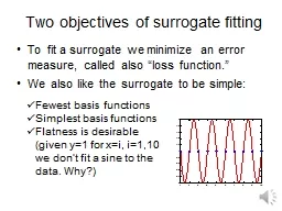
Many applications of statistical analysis involves a continuous variable as dependent variable (DV) but both continuous and categorical variables as independent variables (IV).
Relationship between DV and continuous IVs is linear and the slope remains the same in different groups: ANCOVA.
Different slopes: Full model.
An illustrative data set will make this clear.Slide2
Xuhua Xia
Fitting Several Regression Lines
The muscle strength (MS) depends on the diameter of the muscle fiber and the type of muscle (TM).
Identify DV and IV.
How do we incorporate the qualitative variable in to the model? The dummy variables.
TM D MS
A 1 11.5
A 2 13.8
A 3 14.4
A 4 16.8
A 5 18.7
B 1 10.8
B 2 12.3
B 3 13.7
B 4 14.2
B 5 16.6
C 1 13.1
C 2 16.2
C 3 19.0
C 4 22.9
C 5 26.5Slide3
Xuhua Xia
Two Scenarios
Same intercept Different intercepts
Different slopes: full model Same slope: ANCOVASlide4
Xuhua Xia
Two Scenarios
Same intercept Different intercepts
Different slopes Same slope
Y
1
= a + b
1
X
Y
2
= a + b
2 XY
1
- Y
2
= (b
1-b2)X
Y1 = a1 + b XY2 = a2 + b XY1 - Y2 = a1-a2
Multiplicative
effect
Additive
effectSlide5
Xuhua Xia
Plot of MS vs D by TMSlide6
Objectives
Obtain regression equations relating MS to D for each TM.
Compare the mean MS for the three TMs at a given level of D.
Is it meaningful to compare the mean MS for the three TMs without specifying the level of D?Slide7
Xuhua Xia
Explaining the
R functions
Every 'factor' variable (TM in our case) used in
lm
model-fitting creates k-1 dummy variable:
DUMA = 0
(not created)
DUMB
= 1 if
TM=B
= 0 otherwise
DUMC
= 1 if
TM=C
= 0 otherwise
MS =
+ 1DUMB + 2DUMC + 3D + 4DUMB*D
+
5DUMC*D + The solution option prints estimates of the model coefficients.Slide8
Xuhua Xia
Illustration with EXCEL
MS
TM
D
DUMB
DUMC
DUMB*D
DUMC*D
11.5
A
1
0
0
0
0
13.8
A
2
0
0
0
0
14.4
A
3
0
0
0
0
16.8
A
4
0
0
0
0
18.7
A
5
0
0
0
0
10.8
B
1
1
0
1
0
12.3
B
2
1
0
2
0
13.7
B
3
1
0
3
0
14.2
B
4
1
0
4
0
16.6
B
5
1
0
5
0
13.1
C
1
0
1
0
1
16.2
C
2
0
1
0
2
19
C
3
0
1
0
3
22.9
C
4
0
1
0
4
26.5
C
5
0
1
0
5Slide9
R functions
md <-
read.table
("
DiffSlopeMuscle.txt
",header
=T)
attach(md)
minX
<-
min(D)
maxX
<-
max(D)
minY
<-
min(MS)
maxY
<-max(MS)plot(D[TM=="A"],MS[TM=="A"],xlab="D",ylab="MS",xlim=c(minX,maxX
),ylim
=c(minY,maxY) ,pch=16)points(D[TM
== "B"], MS[TM == "B"],
col='red',
pch=16)points(D[TM=="C"], MS[TM == "C"], col='blue',
pch
=16)
# Will ANOVA reveal the difference between the three teachers?
fitANOVA
<-
aov
(D~TM);
anova
(
fitANOVA
)
# No significant difference in
D,
so students at the beginning appears
# to be similar. Given the same-quality students to begin with, which
# teacher will produce high-performing students at the end?
fitANOVA
<-
aov
(MS~TM);
anova
(
fitANOVA
)
# Check the plot for slope heterogeneity
# Explicit test of slope heterogeneity
fit<-
lm(MS~D*TM)
anova
(fit)
# Check for significance: if not significant, then do ANCOVA
fit<-lm(MS~D+TM)
anova
(fit)Slide10
R
Output
>
anova
(fit)
Analysis of Variance Table
Response: MS
Df
Sum
Sq
Mean
Sq F value Pr
(>F)
D 1 138.245 138.245 704.534
7.392e-10
TM 2 98.001 49.001 249.720
1.306e-08
D:TM 2 22.481 11.240 57.284 7.595e-06Residuals 9 1.766 0.196 > summary(fit)Coefficients: Estimate Std. Error t value Pr(>|t|)
(Intercept) 9.8200 0.4646 21.137
5.57e-09D 1.7400 0.1401 12.422 5.73e-07TMB -0.3500 0.6570 -0.533 0.6071
TMC -0.3300 0.6570 -0.502 0.6275D:TMB -0.3900 0.1981 -1.969 0.0805
D:TMC 1.6100 0.1981 8.127
1.95e-05highly significant interaction.
MS=9.82+1.74D-0.35B-0.33C-0.39D*B+1.61D*C
A: MS
= 9.82 + 1.74*D
B
: MS =
9.82 + 1.74D-0.35-0.39D
=
9.47 +
1.35*D
C: MS =
9.82 +1.74D-0.33C+1.61D
=
9.49 +
3.35*D
It might help to show regression with dummy variables in EXCELSlide11
Type I and Type III SS
Xuhua Xia
>
anova
(fit)
Analysis of Variance Table
Response: MS
Df
Sum
Sq
Mean
Sq F value Pr(>F) D 1 138.245 138.245 704.534 7.392e-10 ***
TM 2 98.001 49.001 249.720 1.306e-08 ***
D:TM 2 22.481 11.240 57.284 7.595e-06 ***
Residuals 9 1.766 0.196
>
drop1(
fit,~.,test="F")Single term deletionsModel:MS ~ D * TM Df Sum of Sq RSS AIC F value
Pr
(>F) <none> 1.766 -20.090 D 1 30.2760 32.042 21.385 154.294 5.735e-07 ***TM 2 0.0702 1.836 -23.505 0.179 0.839 D:TM 2 22.4807 24.247 15.203 57.284 7.595e-06 ***
Type I SS and F-test
Type III SS and F-testSlide12
R functions
Xuhua
Xia
nd1<-subset(
md,subset
=(TM=="A"))
nd2<-subset(
md,subset
=(TM=="B"))
nd3<-subset(
md,subset
=(TM=="C"))
nd1<-
nd1[order(nd1$D),]
nd2<-
nd2[order(nd2$D),]
nd3<-
nd3[order(nd3$D),]
y1<-predict(fit,nd1,interval="confidence")y2<-predict(fit,nd2,interval="confidence")y3<-predict(fit,nd3,interval="confidence")
par(
mfrow=c(1,3))plot(D[TM=="A"],MS[TM=="A"],xlab="D",ylab
="MS",xlim=c(minX,maxX
),
ylim=c(minY,maxY) ,pch=16)
points(D[TM
==
"B"], MS[TM
==
"B"],
col='red',
pch
=16)
points(D[TM=="C"], MS[TM
==
"C"],
col='blue',
pch
=16)
lines(nd1$D,y1
[,1],col="black")
lines(nd1$D,y1
[,2],col="black")
lines(nd1$D,y1
[,3],col="black")
lines(nd2$D,y2
[,1],col="red")
lines(nd2$D,y2
[,2],col="red")
lines(nd2$D,y2
[,3],col="red")
lines(nd3$D,y3
[,1],col="blue")
lines(nd3$D,y3
[,2],col="blue")
lines(nd3$D,y3
[,3],col="blue")
Call
plot before linesSlide13
95% CI plots
Xuhua Xia