
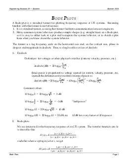
Bode Plots Page 1 A Bode plot is a standard format for plotting frequency response of LTI systems Becoming Since power is propotional to voltage squared or current velocity pressure etc ID: 832569
Download Pdf The PPT/PDF document "Engineering Sciences 22 " is the property of its rightful owner. Permission is granted to download and print the materials on this web site for personal, non-commercial use only, and to display it on your personal computer provided you do not modify the materials and that you retain all copyright notices contained in the materials. By downloading content from our website, you accept the terms of this agreement.


Engineering Sciences 22 Systems Summer
Engineering Sciences 22 Systems Summer 2004 Bode Plots Page 1 A Bode plot is a standard format for plotting frequency response of LTI systems. Becoming (Since power is propotional to voltage squared (or current, velocity, pressure, etc., decibels (dB) = 2 Common values 10 log 10 log = 20 log1012 = 3 dB half power 10 log 10 log 10 = 20 dB, etc 10 dB for every factor of 10 in power 2. Bode plots We are interested in the frequency response of ))()(())(()(32121pjpjpjzjzjKjHEngineering Sciences 22 Systems Summer 2004 Bode Plot
s Page 2 Thats a product (or quotient)
s Page 2 Thats a product (or quotient) of a bunch of complex numbers. Using polar form, we can say that the angle of the product (quotient) is the sum of the angles of each term (except for division we subtract, so its the sum of the angles for the top terms, minus the sum of the angles for the terms Summing terms is easy to do grapthe product turns into a sum. Thus, if we plot ththe plots to find the total behavior. For the poles, we could either plot the behavior of (The general plan for how to sketch a Bode plot by hand is, then, to first gain an understa
nding of what individual poles and indiv
nding of what individual poles and individual zeros do, and then add the responses together. It is easiest to understand complex poles and zeros by looking at the response of a complex conjugate pair, rather than trying to look at the complex poles or zeros individually. This handout includes some information on complex pairs, but you arent required to learn how to sketch a Bode plot The following pages contain, first, a catalog of responses you can expect from individual poles and zeros, and then step-by-step instructions on how to construct a Bode plot from
a transfer The examples given on the fol
a transfer The examples given on the following pages all have a normalized (unitless) frequency scale, i.e. /a where a is the pole or zero, and = 2, rather than the usual frequency scale in Hz. The idea is that the point labeled 1 on the plot will appear at the frequency corresponding to the Engineering Sciences 22 Systems Summer 2004 Bode Plots Page 4 2.2 Single zero, -2-1012010203040-2-101204590Magnitude (dB)Phase (deg) Low-frequency asymptote ( Breakpoint at High frequency asymptote, +20 dB/decade Actual curve is +3 dB abov
e breakpoint Low frequency asymptote
e breakpoint Low frequency asymptote = 0° +45° at breakpoint ( High frequency asymptote = +90° Not required for EEngineering Sciences 22 Systems Summer 2004 Bode Plots Page 6 3. Second order underdamped response (for reference onlynot required knowledge for 22) 3.1 Two poles, underdamped, (j) H(j = 290° 40 dB/decade 180° -40-20Gain (dB) = 0.5 = 0.15 = 0.0510-180-135-90-45Normalized Frequency Phase (degrees)Engineering Sciences 22 Systems Summer 2004 Bode Plots Page 8 Identify breakpoints: distance of poles
and zeros from the origin. Mark those o
and zeros from the origin. Mark those on the Start at one of the asymptotes that is constant. (see below if neither is constant). Move along in frequency until you get to a breakpoint. Each breakpoint is associated with a slope of +/-20 dB/decade (+/-6 dB/octave). From left to right, a zero produces an increase in slope (The increase could be from negative to less negative, or from positive to more positive, etc.) Each pole produces a decrease in slope. Work through all the breakpoints, Sketch in a smoother curve, 3 dB below or above each breakpoint (unless
it is a double pole Now fill in the phas
it is a double pole Now fill in the phase by the samethe limit of H(j 0 or infinity. If the limit is real, the phase is 180 degrees or If the limit is zero, you have to look at what direction it came in to zero from. If it came from a positive imaginary number, the phase is 90 degree; a negative imaginary number -90 degrees. If it came from a positive real number, the phase is 0, and if it came from a negative real number, the phase is -90° Then from left to right, each pole causes a 90° transition in phase, and every zero causes a +90° transition in phase.
You can use in phase. You can use ()(
You can use in phase. You can use ()() �HF limit: s/100 - 0 �LF limit: s/(s2) - 0 with breakpoints at 1/(2Instead of starting at HF or LF asymptotes, you can start with the flat center part. Consider ��the approximate value there, where s1 and sthe transfer function, putting the negligible stuff in a small font: H(s) = s/[(s+1)(s+100)] Then. Thus, we can approximate H(s) as s/[100s] = 1/100 or 40 dB in the flat middle part. Then we can start there and sketch the rest. (It slopes down with +/- 20 dB/decade slope on either side