
With a widefield multiIFU spectrograph Cluster studies Clusters provide large samples of galaxies in a moderate field Unique perspective on the interaction of galaxies with their environment As they operate much as a closed box they are useful as tracers of galaxy evolution and of cosmology ID: 292537
Download Presentation The PPT/PDF document "Clusters of galaxies" is the property of its rightful owner. Permission is granted to download and print the materials on this web site for personal, non-commercial use only, and to display it on your personal computer provided you do not modify the materials and that you retain all copyright notices contained in the materials. By downloading content from our website, you accept the terms of this agreement.


Slide1
Clusters of galaxies
With a wide-field multi-IFU spectrographSlide2
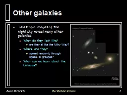
Cluster studies
Clusters provide large samples of galaxies in a moderate field
Unique perspective on the interaction of galaxies with their environment
As they operate much as a closed box, they are useful as tracers of galaxy evolution and of cosmologySlide3
Premise
We will propose a multi-IFU instrument useful for the study of galaxies in clustersSlide4
Key design requirement parameters
Field of View
Spectral resolution
Wavelength coverage
Efficiency or throughput
Crowding restrictions (
fibre
bundle collisions)
Number of
IFUs
Number of elements per IFU
Reconfiguration timeSlide5
Competitors/references
Keck/DEIMOS; Keck/LRIS (
multislits
)
VLT/KMOS (infra-red)
MMT/
Hectospec
(single
fibre
)
AAT/
AAOmega
(single
fibre
)
VLT/Giraffe
15 IFU + 15 sky
Each IFU is only 20 elements, 3x2
arcsec
, 0.5
arcsec
pixels.Slide6
Cluster sizes
Redshift
z
= 0.003 (Virgo) to 1.4, WHT will operate at the low end of this.
Core radius ~1.5
o
for Virgo, ~7
arcmin
for Coma, to a few
arcseconds
.
Virial
radius (normally taken as the radius at which the density is 200
x
ambient) is ~2
Mpc
for rich clusters (1.2
o
at Coma)
1.5 degree diameter field would match
virial
radius at z~0.035.Slide7
Cluster types
Classified by:
Richness
Concentration
Dominance of central galaxy (
Bautz
-Morgan)
Morphology (Rood-
Sastry
) –
cD
, B, L, C, I, F
Galaxy Content (elliptical rich, spiral rich etc)
X-ray structure
Clusters present a wide range of environmentsSlide8
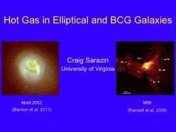
Cluster Types
From Craig
SarazinSlide9
A2151 – BM III
A1656 – BM II
A1367 – BM II-III
A2199 – BM ISlide10
What do we want to know
Mass profiles
Galaxy properties
Luminosity function
Stellar content
Evolution with
redshift
of these properties
Effect of environment upon galaxy:
Morphology
Current star formation
Dynamical state (e.g. tidal truncation)Slide11
Cluster evolution
Necessity of low
redshift
samples in clusters of all types.
Easy to get 8-10
m
time for high-
redshift
clusters, but not for the
vital
low-
redshift
comparisons.
WHT is best employed making sure we understand the low-
redshift
population.Slide12
Science measurements
Absorption lines
Spatially resolved kinematics
Velocity (for
membership),Velocity
dispersions, Fundamental Plane
Line strengths
Ages,
metallicity
, epoch of last star formation, ”Z-planes”
Emission lines
Spatially resolved kinematics
Tully-Fisher relation
Ram pressure or tidally induced star formation
Fluxes or equivalent widths
Metallicity
in galaxies and intra-cluster gasSlide13
Examples:
Examples from recent work
How can WHT contribute when there are larger telescopes around?
What are the requirements?Slide14
Example – Fundamental plane and Faber-Jackson relation of dwarfs
Ehsan
Kourkchi
et al. – Keck/DEIMOS dataSlide15
Example – Fundamental plane and Faber-Jackson relation of dwarfs
Ehsan
Kourkchi
et al. – Keck/DEIMOS dataSlide16
Requirements for FP/FJ relation
σ
down to 20 km/
s
requires R ~ 5000 - 7000
λrange
820 – 870 nm and/or 480 – 570 nm
Control over aperture corrections
IFU aperture ~ 10
arcsec
for comparison with Keck etc. observations of clusters at Z ~ 0.5 - 0.8
Samples of tens of galaxies (not hundreds)
Exposures of hoursSlide17
Stellar populations
Estimate 3 parameters: weighted age; [Z/H]; [
α
/Fe] (or [E/Fe]) by fitting line pairs of index measurements onto model grids.
[
α
/Fe] tells you something about the timescale of star formation.
Keck/LRIS data
Scaled Solar
[E/Fe] = +0.3Slide18
Example – Star formation ceased more recently in the outer parts of Coma
Russell Smith et al. using MMT/
HectospecSlide19
Z-planes
4 dimensional space (age, [Z/H], [
α
/Fe],
σ
)
Marginalise
over one parameter and then you have something which looks a bit like the FP.Slide20
Requirements for stellar populations
R ~ 1000
λ
range 390 – 600 nm (820 – 870 nm also useful but not vital)
Field of view ~ 1 degree or more.
Aperture ~ 10
arcsec
if we are comparing with distant clusters
Samples of tens to hundreds of galaxies.Slide21
Example – tidal or ram-pressure induced starbursts
Sakai et al. in
Abell
1367
Anomalously metal rich starbursts?
Hα imagesSlide22
Requirements for emission line diagnostics
R ~ 1000 – 2000
λrange
370 – 700 nm
Field size ~
virial
radius
Aperture 10 - 30
arcsec
Samples of a fewSlide23
Distant clusters (z
~ 0.3 – 0.5)
Postman et al. HST/MCT allocation
524 orbits with ACS and WFC3
24 clusters
z
~ 0.15 – 0.9, in 14
passbands
Headline science is gravitational
lensing
and
supernovae, however far more interesting will be the multiband dataset on the cluster targets themselves.
Spectroscopic
followup
of samples selected on
colours
and morphology.Slide24
Distant clusters (
z
~ 0.3 – 0.5)
EDisCS
ESO Distant Cluster Survey
Identification, deep photometry and spectroscopy of 10 clusters around
z
~ 0.5 and 10 around
z
~ 0.8
Spectroscopy is FORS2 (R ~ 1200)
Science goals are build up of stellar populations with
redshift
(plus weak
lensing
).Slide25
However:
In general spectroscopic
followup
will use larger (8-10m) telescopes.
Better with single
fibres
, with more attention paid to how close you could position them to each other.
Alternative is large single IFU covering whole cluster core
Moves required spectral coverage for same science goals
redwards
.Slide26
Example – Evolution of the Tully-Fisher relation
Originally a distance indicator, now a tool for measuring evolution of galaxy luminosity
Correlation between
V
max
and absolute magnitude
Originally
V
max
from HI single beam measurements
Optical
V
max
measured with
Hαline
Aperture has to be large enoughSlide27
Optical Tully-Fisher relation
From
Stéphane
Courteau
Top horizontal axis is in
kpc
Require to get out to 10 – 20
kpcSlide28
Tully-Fisher relation at
z
~ 0.3 – 0.5
Metevier
et al. in Cl0024 at
z
~ 0.4. Keck/LRIS data
Find galaxies
underluminous
with respect to local T-F relationSlide29
Requirements for T-F evolution
Aperture must be 20 – 40
kpc
diameter, equal to 4.8 – 9.6
arcsec
at
z
= 0.2.
R ~ 1000
λrange
780 – 990 nm (Hα at
z
= 0.2 - 0.5)
Field size 5 - 15
arcminutes
Samples of 10 - 30Slide30
Key design requirement parameters
Field of View
1.5
o
; 1
o
minimum
Spectral resolution
R = 1000 - 7000
Wavelength coverage
λ
= 370 – 990 nm
Crowding
restrictions (
fibre
bundle collisions)
2-3
x
aperture size
Number of
IFUs
Minimum 30
Number of elements per IFU
100 (10
x
10
arcsec
)
Reconfiguration time
not critical