/
Fitting Fitting We’ve learned how to detect edges, corners, blobs. Now what? Fitting Fitting We’ve learned how to detect edges, corners, blobs. Now what?

Fitting Fitting We’ve learned how to detect edges, corners, blobs. Now what? - PowerPoint Presentation

jewelupper
jewelupper . @jewelupper
Follow
346 views
Uploaded On 2020-06-23

Fitting Fitting We’ve learned how to detect edges, corners, blobs. Now what? - PPT Presentation

We would like to form a higherlevel more compact representation of the features in the image by grouping multiple features according to a simple model Source K Grauman Fitting Choose a parametric model ID: 784177

line model fitting points model line points fitting squares ransac source number select parameters outliers sample hypothesize robust function

Share:

Link:

Embed:

Download Presentation from below link

Download The PPT/PDF document "Fitting Fitting We’ve learned how to d..." is the property of its rightful owner. Permission is granted to download and print the materials on this web site for personal, non-commercial use only, and to display it on your personal computer provided you do not modify the materials and that you retain all copyright notices contained in the materials. By downloading content from our website, you accept the terms of this agreement.


Presentation Transcript

Slide1

Fitting

Slide2

Fitting

We’ve learned how to detect edges, corners, blobs. Now what?

We would like to form a higher-level, more compact representation of the features in the image by grouping multiple features according to a simple model

Slide3

Source: K. Grauman

Fitting

Choose a

parametric model

to represent a set of features

simple model: lines

simple model: circles

complicated model: car

Slide4

Fitting: Challenges

Noise

in the measured feature locations

Extraneous data:

clutter (outliers), multiple lines

Missing data: occlusions

Case study: Line detection

Slide5

Fitting: Overview

If we know which points belong to the line, how do we find the “optimal” line parameters?

Least squares

What if there are outliers?

Robust fitting, RANSAC

What if there are many lines?

Voting methods: RANSAC, Hough transformWhat if we’re not even sure it’s a line?Model selection (not covered)

Slide6

Least squares line fitting

Data:

(

x

1

, y

1), …, (xn, yn)Line equation: y

i

= m

x

i

+ b

Find (

m

,

b

) to minimize

Normal equations:

least squares solution to

XB=Y

(

x

i

,

y

i

)

y=mx+b

Slide7

Problem with “vertical” least squares

Not rotation-invariant

Fails completely for vertical lines

Slide8

Total least squares

Distance between point

(

x

i

, y

i) and line ax+by=d (a

2

+b

2

=

1):

|

ax

i

+

by

i

– d

|

(

x

i

,

y

i

)

ax+by=d

Unit normal:

N=

(

a, b

)

Slide9

Total least squares

Distance between point

(

x

i

, y

i) and line ax+by=d (a

2

+b

2

=

1):

|

ax

i

+

by

i

– d

|

Find

(

a

,

b

,

d

)

to minimize the sum of squared perpendicular distances

(

x

i

,

yi)ax+by

=d

Unit normal:

N=

(a, b)

Slide10

Total least squares

Distance between point

(

x

i

, y

i) and line ax+by=d (a

2

+b

2

=

1):

|

ax

i

+

by

i

– d

|

Find

(

a

,

b

,

d

)

to minimize the sum of squared perpendicular distances

(

x

i

,

yi)ax+by

=d

Unit normal:

N=

(a, b)

Solution to (

U

T

U

)

N =

0,

subject to

||

N

||

2

= 1

: eigenvector of

U

T

U

associated with the smallest eigenvalue (least squares solution

to

homogeneous linear system

UN

=

0

)

Slide11

Total least squares

second moment matrix

Slide12

Total least squares

N

= (

a

,

b

)

second moment matrix

F&P (2

nd

ed.) sec. 22.1

Slide13

Least squares as likelihood maximization

Generative model

: line points are sampled independently and corrupted by Gaussian noise in the direction perpendicular to the line

(

x

,

y

)

ax+by=d

(

u

,

v

)

ε

point on the line

noise:

sampled from

zero-mean

Gaussian with

std. dev.

σ

normal

direction

Slide14

Least squares as likelihood maximization

Likelihood

of points given line parameters (

a

,

b

, d):

Log-likelihood:

(

x

,

y

)

ax+by=d

(

u

,

v

)

ε

Generative model

: line points are sampled independently and corrupted by Gaussian noise in the direction perpendicular to the line

Slide15

Least squares: Robustness to noise

Least squares fit to the red points:

Slide16

Least squares: Robustness to noise

Least squares fit with an outlier:

Problem: squared error heavily penalizes outliers

Slide17

Robust estimators

General approach: find model parameters

θ

that minimize

r

i (xi, θ) – residual of

ith

point

w.r.t

. model parameters

θ

ρ

robust function

with scale parameter

σ

The robust function

ρ

behaves like squared distance for small values of the residual

u

but saturates for larger values of

u

Slide18

Robust estimators

General approach: find model parameters

θ

that minimize

r

i (xi, θ) – residual of

ith

point

w.r.t

. model parameters

θ

ρ

robust function

with scale parameter

σ

Robust fitting is a nonlinear optimization problem

that must

be solved iteratively

Least squares solution can be used for initialization

Scale of robust function should be chosen

carefully

Slide19

Choosing the scale: Just right

The effect of the outlier is minimized

Slide20

The error value is almost the same for every

point and the fit is very poor

Choosing the scale: Too small

Slide21

Choosing the scale: Too large

Behaves much the same as least squares

Slide22

RANSAC

Robust fitting can deal with a few outliers – what if we have very many?

Random sample consensus (RANSAC):

Very general framework for model fitting in the presence of outliers

Outline

Choose a small subset of points uniformly at randomFit a model to that subsetFind all remaining points that are “close” to the model and reject the rest as outliers

Do this many times and choose the best modelM. A. Fischler, R. C. Bolles. Random Sample Consensus: A Paradigm for Model Fitting with Applications to Image Analysis and Automated Cartography. Comm. of the ACM, Vol 24, pp 381-395, 1981.

Slide23

RANSAC for line fitting example

Source:

R.

Raguram

Slide24

RANSAC for line fitting example

Least-squares fit

Source:

R.

Raguram

Slide25

RANSAC for line fitting example

Randomly select minimal subset of points

Source:

R.

Raguram

Slide26

RANSAC for line fitting example

Randomly select minimal subset of points

Hypothesize a model

Source:

R.

Raguram

Slide27

RANSAC for line fitting example

Randomly select minimal subset of points

Hypothesize a model

Compute error function

Source:

R.

Raguram

Slide28

RANSAC for line fitting example

Randomly select minimal subset of points

Hypothesize a model

Compute error function

Select points consistent with model

Source:

R.

Raguram

Slide29

RANSAC for line fitting example

Randomly select minimal subset of points

Hypothesize a model

Compute error function

Select points consistent with model

Repeat

hypothesize-and-verify loop

Source:

R.

Raguram

Slide30

30

RANSAC for line fitting example

Randomly select minimal subset of points

Hypothesize a model

Compute error function

Select points consistent with model

Repeat hypothesize-and-verify loop

Source:

R.

Raguram

Slide31

31

RANSAC for line fitting example

Randomly select minimal subset of points

Hypothesize a model

Compute error function

Select points consistent with model

Repeat hypothesize-and-verify loop

Uncontaminated sample

Source:

R.

Raguram

Slide32

RANSAC for line fitting example

Randomly select minimal subset of points

Hypothesize a model

Compute error function

Select points consistent with model

Repeat

hypothesize-and-verify loop

Source:

R.

Raguram

Slide33

RANSAC for line fitting

Repeat

N

times:

Draw

s points uniformly at randomFit line to these s pointsFind inliers

to this line among the remaining points (i.e., points whose distance from the line is less than t)If there are d or more inliers, accept the line and refit using all inliers

Slide34

Choosing the parameters

Initial number of points

s

Typically minimum number needed to fit the model

Distance threshold

tChoose t so probability for inlier is p (e.g. 0.95)

Zero-mean Gaussian noise with std. dev. σ: t2=3.84σ2Number of samples NChoose N so that, with probability p, at least one random sample is free from outliers (e.g.

p

=0.99) (outlier ratio:

e

)

Source: M. Pollefeys

Slide35

Choosing the parameters

proportion of outliers

e

s

5%

10%

20%

25%

30%

40%

50%

2

2

3

5

6

7

11

17

3

3

4

7

9

11

19

35

4

3

5

9

13

17

34

72

5

4

6

12

17

26

57

146

6

4

7

16

24

37

97

293

7

4

8

20

33

54

163

588

8

5

9

26

44

78

272

1177

Source: M. Pollefeys

Initial number of points

s

Typically minimum number needed to fit the model

Distance threshold

t

Choose

t

so probability for inlier is

p

(e.g. 0.95)

Zero-mean Gaussian noise with std. dev.

σ

: t

2

=3.84

σ

2

Number of samples

N

Choose

N

so that, with probability

p

, at least one random sample is free from outliers (e.g.

p

=0.99) (outlier ratio:

e

)

Slide36

Choosing the parameters

Source: M. Pollefeys

Initial number of points

s

Typically minimum number needed to fit the model

Distance threshold

t

Choose

t

so probability for inlier is

p

(e.g. 0.95)

Zero-mean Gaussian noise with std. dev.

σ

: t

2

=3.84

σ

2

Number of samples

N

Choose

N

so that, with probability

p

, at least one random sample is free from outliers (e.g.

p

=0.99) (outlier ratio:

e

)

Slide37

Choosing the parameters

Initial number of points

s

Typically minimum number needed to fit the model

Distance threshold

tChoose t so probability for inlier is p

(e.g. 0.95) Zero-mean Gaussian noise with std. dev. σ: t2=3.84σ2Number of samples NChoose N so that, with probability p, at least one random sample is free from outliers (e.g.

p

=0.99) (outlier ratio:

e

)

Consensus set size

d

Should match expected inlier ratio

Source: M. Pollefeys

Slide38

Adaptively determining the number of samples

Outlier ratio

e

is often unknown a priori, so pick worst case, e.g. 50%, and adapt if more inliers are found, e.g. 80% would yield

e

=0.2 Adaptive procedure:N=∞, sample_count =0While N

>sample_countChoose a sample and count the number of inliersIf inlier ratio is highest of any found so far, set e = 1 – (number of inliers)/(total number of points)Recompute N from e:

Increment the

sample_count

by 1

Source: M. Pollefeys

Slide39

RANSAC pros and cons

Pros

Simple and general

Applicable to many different problems

Often works well in practice

ConsLots of parameters to tuneDoesn’t work well for low inlier ratios (too many iterations, or can fail completely)Can’t always get a good initialization

of the model based on the minimum number of samples

Slide40

Fitting: Review

Least squares

Robust fitting

RANSAC

Slide41

Fitting: Review

If we know which points belong to the line, how do we find the “optimal” line parameters?

Least squares

What if there are outliers?

Robust fitting, RANSAC

What if there are many lines?

Voting methods: RANSAC, Hough transform