
Chapter 8 of Macroeconomics 10 th edition by N Gregory Mankiw ECO62 Udayan Roy PART III Growth Theory The Economy in the Very Long Run The SolowSwan Model This is a theory of macroeconomic ID: 1028384
Download Presentation The PPT/PDF document "Economic Growth I: Capital Accumulation ..." is the property of its rightful owner. Permission is granted to download and print the materials on this web site for personal, non-commercial use only, and to display it on your personal computer provided you do not modify the materials and that you retain all copyright notices contained in the materials. By downloading content from our website, you accept the terms of this agreement.


1. Economic Growth I: Capital Accumulation and Population GrowthChapter 8 of Macroeconomics, 10th edition, by N. Gregory MankiwECO62 Udayan RoyPART III Growth Theory: The Economy in the Very Long Run
2. The Solow-Swan ModelThis is a theory of macroeconomic dynamicsUsing this theory, you can predict where an economy will be tomorrow, the day after, and so on, if you know where it is todayyou can predict the dynamic effects of changes inthe saving ratethe rate of population growthand other factors
3. Two productive resources and one produced goodThere are two productive resources:Capital, KLabor, LThese two productive resources are used to produce onefinal good, Y
4. The Production FunctionThe production function is an equation that tells us how much of the final good is produced with specified amounts of capital and laborY = F(K, L)Example: Y = 5K0.3L0.7Y = 5K0.3L0.7labor0102030capital000001025.0640.7154.072030.8550.1266.573034.8456.6075.184037.9861.7081.95
5. Constant returns to scaleY = F(K, L) = 5K0.3L0.7Note: if you double both K and L, Y will also doubleif you triple both K and L, Y will also triple… and so onThis feature of the Y = 5K0.3L0.7 production function is called constant returns to scaleY = 5K0.3L0.7labor0102030capital000001025.0640.7154.072030.8550.1266.573034.8456.6075.184037.9861.7081.95The Solow-Swan model assumes that production functions obey constant returns to scale
6. Constant returns to scaleDefinition: The production function F(K, L) obeys constant returns to scale if and only iffor any positive number z (that is, z > 0)F(zK, zL) = zF(K, L) Example: Suppose F(K, L) = 5K0.3L0.7.Then, for any z > 0, F(zK, zL) = 5(zK)0.3(zL)0.7 = 5z0.3K0.3z0.7L0.7 = 5z0.3 + 0.7K0.3L0.7 = z5K0.3L0.7 = zF(K, L)At this point, you should be able to do problem 1 (a) on page 232 of the textbook.
7. Constant returns to scaleCRS requires F(zK, zL) = zF(K, L) for any z > 0Let z be 1/L. Then,y = Y/L denotes per worker outputk = K/L denotes per worker stock of capitalSo, y = F(k, 1) .From now on, F(k, 1) will be denoted f(k), the per worker production function.So, y = f(k) .
8. Per worker production function: exampleky001526.15636.95247.57958.10368.55978.96489.33099.666109.9761110.2661210.5371310.7931411.0361511.2671611.4871711.6981811.9001912.0952012.282This is what a typical per worker production function looks like: concaveAt this point, you should be able to do problems 1 (b) and 3 (a) on pages 232 and 233 of the textbook.
9. The Cobb-Douglas Production FunctionY = F(K, L) = 5K0.3L0.7This production function is itself an instance of a more general production function called the Cobb-Douglas Production FunctionY = AKαL1 − α , where A is any positive number (A > 0) and α is any positive fraction (1 > α > 0)
10. Per worker Cobb-Douglas production functionY = AKαL1 − α implies y = Akα = f(k)In problem 1 on page 232 of the textbook, you get Y = K1/2L1/2, which is the Cobb-Douglas production with A = 1 and α = ½. In problem 3 on page 233, you get Y = K0.3L0.7, which is the Cobb-Douglas production with A = 1 and α = 0.3.
11. Per worker production function: graph
12. Income, consumption, saving, investmentOutput = incomeThe Solow-Swan model assumes that each individual saves a constant fraction, s, of his or her incomeTherefore, saving per worker = sy = sf(k)This saving becomes an addition to the existing capital stockConsumption per worker is denoted c = y – sy = (1 – s)y
13. Income, consumption, saving, investment: graph
14. Depreciation But part of the existing capital stock wears outThis is called depreciationThe Solow-Swan model assumes that a constant fraction, δ, of the existing capital stock wears out in every periodThat is, an individual who currently has k units of capital will lose δk units of capital though depreciation (or, wear and tear)
15. DepreciationAlthough 0 < δ < 1 is the fraction of existing capital that wears out every period, in some cases—as in problem 1 (c) on page 219 of the textbook—depreciation is expressed as a percentage.In such cases, care must be taken to convert the percentage value to a fractionFor example, if depreciation is given as 5 percent, you need to set δ = 5/100 = 0.05
16. Depreciation: graph
17. dynamics
18. Dynamics: what time is it?We’ll attach a subscript to each variable to denote what date we’re talking aboutFor example, kt will denote the economy’s per worker stock of capital on date t and kt+1 will denote the per worker stock of capital on date t + 1
19. How does per worker capital change?A worker has kt units of capital on date t He or she adds syt units of capital through savingand loses δkt units of capital through depreciationSo, each worker accumulates kt + syt − δkt units of capital on date t + 1Does this mean kt+1 = kt + syt − δkt?Not quite!
20. Population GrowthThe Solow-Swan model assumes that each individual has n kids in each periodThe kids become adult workers in the period immediately after they are born and, like every other worker, have n kids of their ownand so on
21. Population GrowthLet the growth rate of any variable x be denoted xg. It is calculated as follows:Therefore, the growth rate of the number of workers, Lg, is:
22. How does per worker capital change?Recall that, each individual has kt units of capital on date tand accumulates kt + syt − δkt units of capital on date t + 1which he/she shares equally with his/her n kids(and these kids born at time t are adult workers at time t + 1).Therefore, the per worker capital stock at time t + 1 is:
23. Dynamics: algebraUsing this equation and other information about the production function, population growth and depreciation, we would be able to use information about the current level of k to predict the entire future of the economy!Let’s try an algebraic example.
24. Now we are ready for dynamics!Dynamics: algebraWe also saw earlier that in the Cobb-Douglas case, y = f(k) = Akα.Therefore, we get
25. Dynamics: algebraA =10α =0.3δ =0.1n =0.2k0 =12s =0.2tktyt = Aktαsytδkt01221.074364.2148721.2112.5123921.340384.2680761.251239212.9410221.557114.3114231.294102313.2986221.734124.3468231.329862413.5963221.878954.3757891.359632513.8437321.997634.3995261.384373614.0490722.095014.4190031.404907714.219322.174994.4349991.42193814.3603122.240744.4481471.436031914.4770222.294814.4589621.4477021014.5735722.339314.4678621.457357
26. Dynamics: algebraA =10α =0.3δ =0.1n =0.2k0 =12s =0.2tktyt = Aktαsytδkt01221.074364.2148721.2112.5123921.340384.2680761.251239212.9410221.557114.3114231.294102313.2986221.734124.3468231.329862413.5963221.878954.3757891.359632513.8437321.997634.3995261.384373614.0490722.095014.4190031.404907714.219322.174994.4349991.42193814.3603122.240744.4481471.436031914.4770222.294814.4589621.4477021014.5735722.339314.4678621.457357At this point, you should be able to do problems 1 (d) and 3 (c) on pages 232 and 233 of the textbook. Please give them a try.
27. Dynamics: algebra to graphsAlthough this is the basic Solow-Swan dynamic equation, a simple modification will help us analyze the theory graphically.Now we are ready for graphical analysis.
28. Dynamics: algebra to graphsThis version of the Solow-Swan equation will help us understand the model graphically.
29. Dynamics: algebra to graphs1. The economy grows if and only if per worker saving and investment [sf(kt)] exceeds break-even investment [(δ + n)kt].2. The economy shrinks if and only if per worker saving and investment [sf(kt)] is less than break-even investment [(δ + n)kt].3. The economy is at a steady state if and only if per worker saving and investment [sf(kt)] is equal to break-even investment [(δ + n)kt].4. (δ + n)kt is called break-even investmentThis version of the Solow-Swan equation will help us understand the model graphically.
30. Dynamics: graph
31. Investment and break-even investmentCapital per worker, k sf(kt)(δ + n)ktk* k1Steady state
32. Investment and break-even investmentCapital per worker, k sf(kt)(δ + n)ktk* k1Steady stateBreak-even investmentk1investment
33. Investment and break-even investmentCapital per worker, k sf(kt)(δ + n)ktk* k1Steady statek1k2k1
34. Investment and break-even investmentCapital per worker, k sf(kt)(δ + n)ktk* k1Steady stateBreak-even investmentk2investmentk2
35. Investment and break-even investmentCapital per worker, k sf(kt)(δ + n)ktk* k1Steady statek1k2k2k3k2
36. Steady state: algebra
37. The Steady State: AlgebraThe economy eventually reaches the steady stateThis happens when per worker saving and investment [sf(kt)] is equal to break-even investment [(δ + n)kt].For the Cobb-Douglas case, this condition is:At this point, you should be able to do problems 1 (c) and 3 (b) on pages 232 and 233 of the textbook. Please give them a try.
38. There is no growth!In the long run, saving per worker is constant and equal to sy* = (δ + n)k*. Therefore,Therefore, And consumption per worker is also constant. It is equal to c* = (1 – s)y*
39. Steady State and Transitional Dynamics: algebratktyt = Aktαsytδkt01221.074364.2148721.2112.5123921.340384.2680761.251239212.9410221.557114.3114231.294102313.2986221.734124.3468231.329862413.5963221.878954.3757891.359632513.8437321.997634.3995261.384373614.0490722.095014.4190031.404907714.219322.174994.4349991.42193814.3603122.240744.4481471.436031914.4770222.294814.4589621.4477021014.5735722.339314.4678621.457357A =10α =0.3δ =0.1n =0.2k0 =12s =0.2k* =15.03185
40. Solow-swan predictions for the steady state
41. There is no growth!The Solow-Swan model predicts that Every economy will end up at the steady-state; in the long run, the growth rate is zero!That is, k = k* and y = f(k*) = y* in the long runGrowth is possible—temporarily!—only if the economy’s per worker stock of capital is less than the steady state per worker stock of capital (k < k*)If k < k*, the smaller the value of k, the faster the growth of k and y
42. There is no growth!So, in the long run: Capital per worker, k = k*, is constantOutput per worker, y = f(k*) = y*, is constantSaving (and investment) per worker, sy*, is constantConsumption per worker, c* = y* – sy* = (1 – s)y*, is also constant.
43. The Steady StateIn the long run, the economy ends up at the steady stateOutput, investment and break-even investmentk(δ + n)ktf(k)k*sf(k)c*f(k*)sf(k*)
44. Solow-swan predictions for changes to the steady stateWhat might be the long-run consequences of:The destruction of physical capital (perhaps by war or natural disaster)An increase in the saving rateAn increase in the rate of population growth
45. A sudden fall in capital per workerA sudden decrease in k could be caused by:Earthquake or war that destroys capital but not peopleImmigration A decrease in uWhat does the Solow-Swan model say will be the result of this?
46. Investment and depreciation Capital per worker, k sf(kt)(δ + n)ktk* k1A sudden fall in capital per worker1. A sudden decline2. A gradual return to the steady stateAt this point, you should be able to do problem 2 on pages 235 of the textbook. Please give it a try.Solow-Swan Predictions Gridkt+1, yt+1, Δktk*, y*, i* = sy*c* = (1 – s)y*kt?00
47. An increase in the saving rateInvestment,break-even investmentk(δ + n)kts1f(k)s2f(k)k1*k2*An increase in the saving rate causes a temporary spurt in growth. The economy returns to a steady state. But at the new steady state, per worker capital, output, and saving are all higher. Per worker consumption is a bit trickier.
48. An increase in the saving rateInvestment, break-even investmentk(δ + n)kts1f(k)1. An increase in the saving rate raises investment …2. … causing k to grow (toward a new steady state) s2f(k)k1*k2*3. This raises steady-state per worker output y* = f(k*) and saving sy*.4. The growth rate begins at zero, becomes positive for a while, and eventually returns to zero.
49. An increase in the saving rateInvestment and break-even investmentk(δ + n)ktf(k)k*2. What can we say about the steady state levels of k, y, and c when s = 0?3. And when s = 1?1. Recall that the saving rate, s, is a fraction between 0 and 1.4. So, how is consumption per worker, c, affected by changes in s?sf(k)c*f(k*)sf(k*)
50. Being the grasshopper is not good!Investment and break-even investmentk(δ + n)ktf(k)k*= 02. What can we say about the steady state levels of k, y, and c when s = 0?1. Recall that the saving rate is a fraction between 0 and 1.sf(k) when s = 03. They are all zero!
51. Being a miserly ant is not good either!Investment and break-even investmentk(δ + n)ktf(k)k*2. What can we say about the steady state levels of k, y, and c when s = 1?1. Recall that the saving rate is a fraction between 0 and 1.= sf(k)c*= 0f(k*)sf(k*)
52. Effect of saving on steady state consumption01Saving rate, sSteady state consumption per worker, c* = (1 – s)f(k*)Golden Rule Saving rateGolden Rule consumption per workerFor the Cobb-Douglas case, it can be shown that the Golden Rule saving rate is equal to capital’s share of all income, which is approximately 30% or 0.30.The US saving rate is well below 0.30. So, according to the Solow-Swan model, if we save more we will, in the long run, consume more too!
53. What do we get for thrift?In the long run, a higher rate of saving and investment gives usA higher per worker incomeBut not a faster rate of growthAnd consumption per worker, c* = (1 – s)y*, may increase or decrease or stay unchanged when s increases.At this point, you should be able to do problem 4 on page 233 of the textbook. Please try it.
54. Whole lecture in one slide!Solow-Swan Predictions Gridkt+1, yt+1, Δktk*, y*, i* = sy*c* = (1 – s)y*kt?00s++?A+++n–––δ–––
55. Effect of saving: evidence
56. Faster population growth3. This reduces steady-state per worker output y* = f(k*), saving sy*, and consumption (1 – s)y*.4. The growth rate begins at zero, becomes negative for a while, and eventually returns to zero.5. The effect is the same if depreciation increases
57. What do we get for having fewer kids?In the long run, a lower rate of population growth gives usA higher per worker incomeBut not a faster rate of growthAt this point, you should be able to do problem 6 on page 233 of the textbook. Please try it.
58. Faster population growth: evidenceThis chart, though included in the 9th edition of the course’s textbook, has been dropped from the 10th edition.
59. Alternative perspectives on population growthThe Malthusian Model (1798)Predicts population growth will outstrip the Earth’s ability to produce food, leading to the impoverishment of humanity.Since Malthus, world population has increased sixfold, yet living standards are higher than ever.Malthus neglected the effects of technological progress.
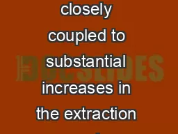
60. Alternative perspectives on population growthThe Kremerian Model (1993)Posits that population growth contributes to economic growth. More people = more geniuses, scientists & engineers, so faster technological progress.Evidence, from very long historical periods: As world pop. growth rate increased, so did rate of growth in living standardsHistorically, regions with larger populations have enjoyed faster growth.
61. Alternative perspectives on population growth: Kremer
62. Robert Solow and Trevor Swan
63. Solow-Swan ModelVideo: https://youtu.be/eVAS-t83Tx0 (Intro to the Solow Model of Economic Growth)Video: https://youtu.be/SljsIacQDbc (Physical Capital and Diminishing Returns)Video: https://youtu.be/LQR7rO-I96A (The Solow Model and the Steady State)Video: https://youtu.be/SVWX4Xjl4Os (Human Capital & Conditional Convergence)
64. Growth and IdeasVideo: https://youtu.be/-yPDlowSL1w (The Solow Model and Ideas)Video: https://youtu.be/1mXBg-BVrJ0 (The Economics of Ideas)Video: https://youtu.be/Jz0VXPPZOiU (Patents, Prizes, and Subsidies)Video: https://youtu.be/Ip2-Qa50uBI (Alex Tabarrok on how ideas trump crises)Video: https://youtu.be/4zhPbYYaV5Y (The Idea Equation)
65. Solow-Swan (Going Deeper)https://youtu.be/IqUuxEQUt4I (The Solow Model 1 - Introduction)https://youtu.be/MmsSIoGtyh4 (The Solow Model 2: Comparative Statics)https://youtu.be/lG4m_4uhZIA (The Solow Model 3 -- Taking the Model to Data)https://youtu.be/S1xRi5JPDaM (The Solow Model 4 - Productivity)