Integrating geologic maps with fault mechanics - PowerPoint Presentation

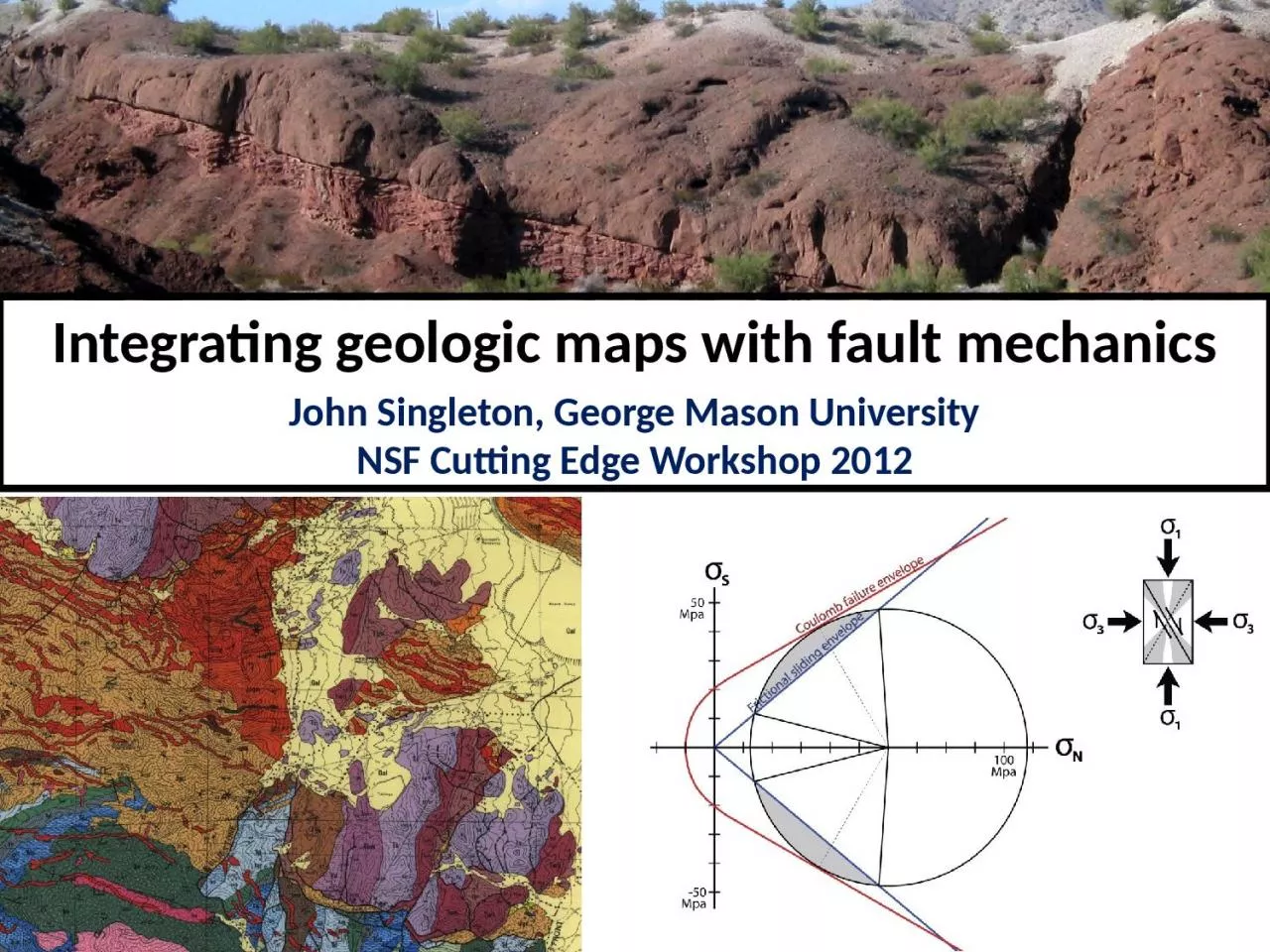
1. Integrating geologic maps with fault mechanicsJohn Singleton, George Mason UniversityNSF Cutting Edge Workshop 2012

2. Exercise overview: • Relate basic stress concepts and fault mechanics (Andersonian theory, Mohr-Coulomb failure, frictional sliding) to geologic maps and cross sections • Part A: students must draw a cross section and make some calculations to explain slip history and mechanics of two generations of normal faults• Part B: interpret the faulting history and the fault mechanics of the Yerington district, Nevada, based on map and cross section by J. Proffett

3. Exercise Goals:• Improve geologic map and cross section skills• Experience stress & fault mechanics problems• Highlight how fault mechanics can help us understand actual geology (not just theory!)• Set stage for lectures on normal faults and paradox of slip on low-angle normal faults

4. Background & materials needed:• Exercise should follow previous lectures and exercises that introduce stress, Mohr circles, Andersonian theory, Coulomb failure, and frictional sliding/Byerlee's law• Ideally should also follow lab/problem set on geologic maps and cross sections• Students will need ruler/protractor, pencil compass, and calculator

5.

6. PART A1) What is the orientation (strike and dip) of the Rattlesnake fault? attitude: N48E, 33°SE (basic three point-type problem from strike lines) 2) Draw a cross section from A-A’ using the topographic profile provided on page 3.  3) What types of faults are the Rattlesnake fault and Jackrabbit fault? normal faults with SE-down displacement 4) Based on your cross section, how much apparent displacement is there on the Rattlesnake fault? On the Jackrabbit fault?~63 m slip on the Rattlesnake fault; ~20 m on the Jackrabbit fault  5) Assuming that these strata were horizontal at the inception of faulting in this area, what was the initial dip of the Rattlesnake fault?strata in hanging wall and footwall are tilted ~27° NW, indicating that Rattlesnake fault restores to ~60° dip (=33°+27°)

7. PART A (continued)As the Rattlesnake fault rotated to its current orientation,friction along the fault increased. The Jackrabbit fault cut through these beds at ~4 km depth after slip on the Rattlesnake fault ceased due to frictional lockup. 6) Assuming an Andersonian stress field, what was the direction and magnitude (in MPa) of σ1 when the Jackrabbit fault formed (at 4 km)? (the average density of these strata is ~2,500 kg/m3).σ1 = vertical (Andersonian theory for normal faulting); vertical stress = lithostatic stress = ρgh = (2,500 kg/m3)*(9.8 m/s2)*(4,000 m) = 98 MPa7) Assuming there was no pore fluid pressure, determine the magnitude and direction of σ3 when the Jackrabbit fault formed (via Mohr-Coloumb failure). Use the Mohr space diagram on page 4 to draw a Mohr circle that illustrates this stress state during formation of the Jackrabbit fault. 8) Now assume that pore fluid pressure was hydrostatic when the Jackrabbit fault formed. What was the magnitude of σ3? Again, illustrate with a Mohr circle.

8. PART A (continued)As the Rattlesnake fault rotated to its current orientation,friction along the fault increased. The Jackrabbit fault cut through these beds at ~4 km depth after slip on the Rattlesnake fault ceased due to frictional lockup. 6) Assuming an Andersonian stress field, what was the direction and magnitude (in MPa) of σ1 when the Jackrabbit fault formed (at 4 km)? (the average density of these strata is ~2,500 kg/m3).σ1 = vertical (Andersonian theory for normal faulting); vertical stress = lithostatic stress = ρgh = (2,500 kg/m3)*(9.8 m/s2)*(4,000 m) = 98 MPa 7) Assuming there was no pore fluid pressure, determine the magnitude and direction of σ3 when the Jackrabbit fault formed (via Mohr-Coloumb failure). Use the Mohr space diagram on page 4 to draw a Mohr circle that illustrates this stress state during formation of the Jackrabbit fault. Mohr circle with σ1 = 98 MPa will intersect Coloumb failure envelope if σ3 = 8 MPa. σ3 = horizontal NW-SE8) Now assume that pore fluid pressure was hydrostatic when the Jackrabbit fault formed. What was the magnitude of σ3? Again, illustrate with a Mohr circle.

9. PART A (continued)As the Rattlesnake fault rotated to its current orientation,friction along the fault increased. The Jackrabbit fault cut through these beds at ~4 km depth after slip on the Rattlesnake fault ceased due to frictional lockup. 6) Assuming an Andersonian stress field, what was the direction and magnitude (in MPa) of σ1 when the Jackrabbit fault formed (at 4 km)? (the average density of these strata is ~2,500 kg/m3).σ1 = vertical (Andersonian theory for normal faulting); vertical stress = lithostatic stress = ρgh = (2,500 kg/m3)*(9.8 m/s2)*(4,000 m) = 98 MPa 7) Assuming there was no pore fluid pressure, determine the magnitude and direction of σ3 when the Jackrabbit fault formed (via Mohr-Coloumb failure). Use the Mohr space diagram on page 4 to draw a Mohr circle that illustrates this stress state during formation of the Jackrabbit fault. Mohr circle with σ1 = 98 MPa will intersect Coloumb failure envelope if σ3 = 8 MPa. σ3 = horizontal NW-SE8) Now assume that pore fluid pressure was hydrostatic when the Jackrabbit fault formed. What was the magnitude of σ3? Again, illustrate with a Mohr circle.Hydrostatic stress at 4 km = (1,000 kg/m3)*(9.8 m/s2)*(4,000 m) = 39.2 MPa. Shift σ1 left by ~39 MPa; Mohr circle with effective σ1 = 59 MPa will intersect Coloumb failure envelope if effective σ3 = -5 MPa, so actual σ3 = 35 MPa (-5+39).

10. PART A (continued) 9) On the Mohr diagram, draw a frictional sliding envelope that accounts for frictional lockup on the Rattlesnake fault at its current orientation, assuming hydrostatic pore fluid pressure. Based on the slope of this envelope, what is the coefficient of friction for the Rattlesnake fault? How does this value compare to Byerlee’s experimental values? If the Rattlesnake fault obeyed Byerlee’s law (σs=0.85*σn), what would have been the dip of the fault when it locked up?Draw a frictional sliding envelope that intersects the Mohr circle (from question 8) at 2Ѳ=66° (assuming the Rattlesnake fault locked up at ~33°). The slope of this envelope is ~36°, corresponding to a coefficient of friction of 0.73 (μ = tan φ = tan 36 = 0.73). This is about 14% less than the average coefficient of friction determined from Byerlee’s experiments (0.85). If the Rattlesnake fault obeyed Byerlee’s law, it would have locked up at ~37°.

11. Part B: Geologic map & cross section of the Yerington district, Nevada (J. Proffett)

12. Proffett, 1977 (GSAB)

13. 10) What kind of faulting has occurred here?   normal faulting11) Based on cross-cutting relationships, give the name and orientation of one of the oldest faults exposed near A-A’. Give the name and orientation of one of the youngest faults. Oldest: Singatse fault; dips ~10-13° E to ENE on map; inferred to be subhorizontal beneath Singatse Peak Youngest: Montana-Yerrington fault, Sales fault, or Range Front fault; all dip ~53-65° E based on map attitudes & cross section12) Which generation of faults have the most displacement? What is the largest amount of displacement on any individual fault? The oldest generation has the most displacement; the largest fault is the Singatse fault with ~4,000 m displacement.

14. 13) Assuming the oldest faults formed when the Tertiary volcanic and sedimentary rocks in the area were horizontal, what was the approximate initial dip of the oldest faults? (hint: determine the average bedding orientation in the fault hanging wall and footwall and restore to horizontal). Is this initial dip consistent with Andersonian theory? Bedding in footwall and hanging wall of Singatse fault mostly dips ~45-55° W, indicating that the Singatse fault initiated at a dip of ~50-65°E. Yes, this is roughly consistent with Andersonian theory.14) Assuming the second generation of faults (e.g. near Singatse Peak) obeyed Andersonian mechanics (and have rotated to its current orientation), at what angle did the oldest generation of faults cease to slip? At what angle did the second generation of faults cease to slip? Are these angles roughly consistent with Byerlee’s law (where σs=0.85*σn)? (e.g. see your answer to question 9 in Part A) The second generation of faults dip ~23-28°E where they cut the subhorizontal Singatse fault. If these faults initiated with an Andersonian ~60° dip, they must have cut the Singatse fault when it dipped ~32-37°. This second generation of faults are cut by the youngest generation of faults, which mostly dip ~50-60° E. Assuming this youngest generation initiated with a ~60° dip, the second generation of faults became inactive and were cut when they dipped ~25-35°. These angles suggest coefficients of sliding friction slightly lower than Byerlee’s law (e.g. lockup at ~37° for conditions given in question 9).

15. Byerlee, 197815) In his 1977 paper published on this area, Proffett indicates that clay gouge is present along faults in this area. In addition, based on structural reconstructions, the Singatse fault in this area must have been >10 km deep where it was cut by younger faults. Given this information, why may the fault lockup angles you inferred in question 14 differ from those predicted by the relationship σs=0.85*σn? Take a look at Byerlee’s experimental data below. Clay has a lower coefficient of friction than most rocks (see clay data points in plot below), so the development of clayey gouge will tend to weaken faults, allowing the normal faults to slip at lower angles. Also, the coefficient of friction decreases to ~0.6 above 200 MPa (2 kbar). The effective σn on the oldest generation of faults may have been ≥200 MPa, allowing the faults to slip at lower angles than that predicted by a coefficient of friction of 0.85.

16. Building on the exercise: • Sets stage for lecture/discussion on styles of extension and slip on low-angle normal faults - Lack of seismicity on normal faults <30° is consistent w/ Andersonian mechanics and μ = 0.6, but there is compelling geologic evidence for slip on low-angle normal faults. How is this mechanically possible?Compilation of active normal fault dips determined from >M 5.5 earthquakesSlip on low-angle normal faults (detachment faults and metamorphic core complexes)Collettini & Sibson, 2001