

Disclaimer I am not an expert When conducting any statistical analysis it is important to evaluate how well the model fits the data and that the data meet the assumptions of the model There are numerous ways to do this and a variety of statistical tests to evaluate deviations from model assum ID: 595519
Download Presentation The PPT/PDF document "What is normal anyway?!" is the property of its rightful owner. Permission is granted to download and print the materials on this web site for personal, non-commercial use only, and to display it on your personal computer provided you do not modify the materials and that you retain all copyright notices contained in the materials. By downloading content from our website, you accept the terms of this agreement.


Slide1
What is normal anyway?!Disclaimer: I am not an expert!Slide2
When conducting any statistical analysis it is important to evaluate how well the model fits the data and that the data meet the assumptions of the model.
There are numerous ways to do this and a variety of statistical tests to evaluate deviations from model assumptions. Slide3
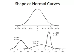
QQ PLOTSTest for normalityRanked samples from our distribution plotted against a similar no. of ranked quantiles taken from a ND
1,6,9 good Slide4
A residual plot
is a graph that shows the
residuals
on the vertical axis and the independent variable on the horizontal axis.
If the points in a
residual plot
are randomly dispersed around the horizontal axis, a linear regression model is appropriate for the data – uncorrelated
Constancy of varianceSlide5
It means that when you plot the individual error against the predicted value, the variance of the error predicted value should be constant. See the red arrows in the picture below, the length of the red lines (a proxy of its variance) are the same.Slide6
Constancy of varianceno heteroscedasticity of residuals=this means that the variance of residuals should not increase with fitted values of response variable
.
Residuals -essentially the distance of the data points from the fitted regression lineSlide7
Idealised examples : Residuals V fitted valuesSlide8
residuals appear exhibit homogeneity, normality, and independence. Those are pretty clear, although I’m not sure if the variation in residuals associated with the predictor (independent) variable Month is a problem. This might be a problem with heterogeneitySlide9
Bad Slide10
sop<-lmer(log(subnatcov+1)~iapcov+avmoisture+loi+cov+P+ss+channel.slope+domnatcov+iapcov:avmoisture+iapcov:cov+(1|river)+(1|trans), data=finalscale, REML=FALSE)Slide11Slide12Slide13Slide14
BetterSQRT transformSlide15
sop<-lmer(sqrt(subnatcov+1)~iapcov+avmoisture+loi+cov+P+ss+domnatcov+channel.slope+(1|river)+(1|trans), data=finalscale, REML=FALSE)Slide16Slide17Slide18Slide19
GLMER: Should we check the spread of points for the random effect? HomogeneitySlide20
No transformationsLayered abundance datamod<-lmer(abundance~iapcov+avmoisture+loi+cov+P+ss+domnatcov+slope
+(
1|river),
data=
finalscale
, REML=FALSE)Slide21Slide22Slide23Slide24Slide25