PPT-Cost-effective Outbreak Detection in Networks

Author : min-jolicoeur | Published Date : 2015-09-19

Jure Leskovec Andreas Krause Carlos Guestrin Christos Faloutsos Jeanne VanBriesen Natalie Glance Scenario 1 Water network Given a real city water distribution network

Presentation Embed Code

Download Presentation

Download Presentation The PPT/PDF document "Cost-effective Outbreak Detection in Net..." is the property of its rightful owner. Permission is granted to download and print the materials on this website for personal, non-commercial use only, and to display it on your personal computer provided you do not modify the materials and that you retain all copyright notices contained in the materials. By downloading content from our website, you accept the terms of this agreement.

Cost-effective Outbreak Detection in Networks: Transcript

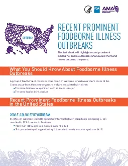
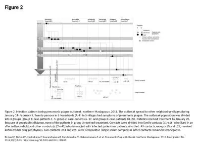
Jure Leskovec Andreas Krause Carlos Guestrin Christos Faloutsos Jeanne VanBriesen Natalie Glance Scenario 1 Water network Given a real city water distribution network And data on how contaminants spread in the network. E. coli . O104:H4 heralds a new paradigm in responding to disease threats. Nicola J. Holden. Leighton Pritchard. EHEC O104:H4 outbreak, Europe 2011. Unprecedented:. scale of outbreak. (3950 affected, 53 deaths; multiple. Sponsored by. Navy and Marine Corps Public Health Center. U.S. Army Public Health Command. Air Force School of Aerospace Medicine. Presented on 27 March 2012 . by . Asha. . Riegodedios. , Staff Epidemiologist, NMCPHC. Please help yourself to breakfast. Please sign-in on the attendance sheet. Please find your seat (names listed on table tents). Applied Outbreak Investigation. Presented by. [Names and agencies]. [Date and location]. Naira Dekhil. 1. , . Besma. Mhenni. 1. , Raja Haltiti. 2. , and . Helmi. Mardassi. 1. . (speaker). . 1. Unit of Typing & Genetics of . Mycobacteria. , . Institut. Pasteur de Tunis, . Tunisia. illness occur from the same organism and are associated with eitherThe same food service operation such as a restaurant orThe same food or drink productIn 2006 an outbreak linked to spinach contaminat Karen Hoover, MD, MPH. Centers for Disease Control and Prevention. July 24, 2019. No conflicts of interest to report. Disclosures. Diagnoses of HIV Infection among Adults and Adolescents, by Transmission Category, 2004–2016—United States and 6 Dependent Areas. Kerrigan McCarthy. Consultant Pathologist. National Institute for Communicable Diseases. 25 June 2020. Source:. Will be on the NICD website from 26 June 2020 in the COVID-19 section. COVID-19 outbreaks in health care facilities . Karoon. . Chanachai. Bureau of Disease Control and Veterinary Service. Department of Livestock Development, Thailand. An event (1). On 28 May 2009, you were still at your work, when an email from your counterpart at the National Institute of Animal Health (NIAH) popped up. In an attachment, you found an official laboratory report from the Upper Northern Regional Veterinary Research and Diagnostic Center. It was a laboratory confirmed case of classical swine fever (CSF) in Mae . San Francisco Bureau C. SHEPARD Mumps Can Occur Even Among theVaccinated, Recent Outbreak ProvesBY TIMOTHY F.KIRN umps outbreaks can occur even amonghighly vaccinated populations, accordingto a report NBS. . ID. NBS. . Label. Description. Coding. for. . T. ransmissio. n. . to. . NNDSS. INV150. OUTBREAK. Outbreak-. associated. Indicates . whether . the case-report . was. . associated. . with. GP session. Bron . McCrae. Deputy Director Healthy Living and Ageing. bmccrae@hnc.org.au. 0447 113 823 . First steps. Building a framework together. Working party . Agreed approaches. Standardising for an emergency . Richard V, Riehm JM, Herindrainy P, Soanandrasana R, Ratsitoharina M, Rakotomanana F, et al. Pneumonic Plague Outbreak, Northern Madagascar, 2011. Emerg Infect Dis. 2015;21(1):8-15. https://doi.org/10.3201/eid2101.131828. Emilio Gonzales. Overview. Why Report. What Is Considered an Outbreak. Response Protocol. Discussion of Current Reporting Method. Review. ●. ●. ●. ●. ●. Why. What. Response. Discussion. Terms to Note. TABLE TOP . EXERCISE. Developed by the . Colorado Integrated Food Safety Center of Excellence. After completing this case study, . students . should be able to. :. Explain what constitutes a foodborne illness outbreak..

Download Document

Here is the link to download the presentation.
"Cost-effective Outbreak Detection in Networks"The content belongs to its owner. You may download and print it for personal use, without modification, and keep all copyright notices. By downloading, you agree to these terms.