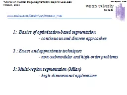
continuous and discrete approaches 2 Exact and approximate techniques nonsubmodular and highorder problems 3 Multiregion segmentation Milan highdimensional applications ID: 333184
Download Presentation The PPT/PDF document "1: Basics of optimization-based segment..." is the property of its rightful owner. Permission is granted to download and print the materials on this web site for personal, non-commercial use only, and to display it on your personal computer provided you do not modify the materials and that you retain all copyright notices contained in the materials. By downloading content from our website, you accept the terms of this agreement.
Slide1
1: Basics of optimization-based segmentation - continuous and discrete approaches 2 : Exact and approximate techniques - non-submodular and high-order problems3: Multi-region segmentation (Milan) - high-dimensional applications
Tutorial on Medical Image Segmentation: Beyond Level-SetsMICCAI, 2014
W
estern UniversityCanada
www.csd.uwo.ca/faculty/yuri/miccai14_MISSlide2
Introduction to Image Segmentationimplicit/explicit representation of boundariesactive contours, level-sets, graph cut, etc.Basic low-order objective functions (energies)physics, geometry, statistics, information theorySet functions, submodularityExact methodsApproximation methodsHigher-order and non-submodular objectivesComparison to gradient descent (level-sets) Part 1Part 2Slide3
ThresholdingTSlide4
ThresholdingS={ p : Ip < T }TSlide5
Background Subtraction?Thresholding-=I= I
obj
- I
bkg
Threshold intensities above
T
better segmentation?Slide6
Good segmentation S ?Objective function must be specified Quality function Cost function Loss function E(S) : 2P “Energy” Regularization functionalSegmentation becomes an optimization problem: S = arg min E(S) Slide7
Good segmentation S ?combining different constraintse.g. on region and boundary Objective function must be specified Quality function Cost function
Loss function
E(S) = E1
(S)+…+ En(S)
“Energy”
Regularization functional
Segmentation becomes an
optimization problem
:
S =
arg
min E(S) Slide8
Beyond linear combination of termsRatios are also usedNormalized cuts [Shi, Malik, 2000]Minimum Ratio cycles [Jarmin Ishkawa, 2001]Ratio regions [Cox et al, 1996]Parametric max-flow applications [Kolmogorov et al 2007]Not in this tutorialSlide9
Segmentation principlesBoundary seedsLivewire (intelligent scissors)Region seedsGraph cuts (intelligent paint)Distance (Voronoi-like cells)Bounding boxGrabcut [Rother et al]Center seedsStar shape [Veksler]Many other options…Normalized cuts [Shi Malik]Mean-shift [Comaniciu]
MDL [Zhu&Yuille
]
Entropy of appearance
interactive vs. unsupervised
Add enough constraints:
Saliency
Shape
Known appearance
TextureSlide10
Boundary seedsLivewire (intelligent scissors)Region seedsGraph cuts (intelligent paint)Distance (Voronoi-like cells)Bounding boxGrabcut [Rother et al]Center seedsStar shape [Veksler]Many other options…Normalized cuts [Shi Malik]Mean-shift [Comaniciu]MDL
[Zhu&Yuille]
Entropy of appearance
interactive vs. unsupervised
Add enough constraints:
Saliency
Shape
Known appearance
Texture
1. We won’t cover everything…
2. We will not emphasize the differences between interactive and unsupervised
(too easy
to convert one into the other)Slide11
optimization-based
Common segmentation techniques
region-growing
intelligent scissors
(live-wire)
active contours
(snakes)
watersheds
boundary-based region-based both region & boundary
thresholding
geodesic
active contours
(e.g. level-sets)
MRF
(e.g. graph
-
cuts)
random walkerSlide12
Common surface representationsmeshlevel-setsgraph labelingon complex
on grid
point cloud
labeling
continuous
optimization
mixed
optimization
combinatorial
optimizationSlide13
Active contours (e.g. snakes)[Kass, Witkin, Terzopoulos 1987]Given: initial contour (model) near desirable object Goal: evolve the contour to fit exact object boundary Slide14
5-14Tracking via active contoursTracking Heart VentriclesSlide15
5-15Active contours - snakes Parametric Curve Representation (continuous case) A curve can be represented by 2 functions open curveclosed curveparameterSlide16
5-16Snake Energyinternal energy encourages smoothness or any particular shapeexternal energy encourages curve onto image structures (e.g. image edges)Slide17
5-17Active contours - snakes (continuous case)internal energy (physics of elastic band)external energy (from image)elasticity / stretchingstiffness / bending
proximity to image edgesSlide18
Active contours – snakes (discrete case)
elastic energy
(elasticity)
bending energy
(stiffness)Slide19
5-19Basic Elastic Snakecontinuous casediscrete case
elastic smoothness term
(interior energy)
image data term
(exterior energy)Slide20
5-20Snakes - gradient descentsimple elastic snake energy
update
equation for
the whole snake
C
here,
energy
is a function of
2n variables
CSlide21
5-21Snakes - gradient descentsimple elastic snake energy
update
equation for each node
C
here,
energy
is a function of
2n variables
CSlide22
5-22Snakes - gradient descentenergy function E(C) for contours C
E(C)
gradient descent steps
local minima
for E(C)
second derivative of image intensities
step size
could be trickySlide23
Implicit (region-based) surface representation via level-sets(implicit contour representation) [Dervieux, Thomasset, 79, 81] [Osher, Sethian, 89]Slide24
Implicit (region-based) surface representation via level-sets[Dervieux, Thomasset, 79, 81] [Osher, Sethian, 89]
The scaling by is easily verified in one dimension
Normal
contour motion can be represented by evolution of level-set function
u
Note 2
:
- level sets
can not
represent
tangential
motion of contour
points ???
Note 1
: - commonly used for gradient descent evolutionSlide25
Tangential vs. normal motion of contour points- normal motion of a contour point visibly changes shape (geometry)- tangential motion generates no “visible” shape changeA simple example of tangential motion of contour points
(rotation)
A simple example of
normal motion
of contour points
(expansion)
Comments: -
geometric “energy” of a contour measures “visible” shape properties
(
length
,
curvature
,
area
,
e.t.c
.). Thus, gradient descent
w.r.t
. geometric objective generates only ”visible” (normal) motion.
level sets can represent contour gradient descent evolution
only for geometric “energies”
E(C)
(
s.t
.
E
is collinear with contour normal )
Level sets
(implicit contour representation)
Geodesic
active contoursSlide26
Tangential vs. normal motion
of contour points
- normal motion of a contour point visibly changes shape (geometry)
- tangential motion generates no “visible” shape change
Parametric contours
(explicit contour representation)
Physics-based
active contours
Comments: -
gradient descent for physics-based “energy” of a contour (e.g.
elasticity
)
may produce geometrically “invisible” tangential motion of contour points
physics-based energy of a contour depends on its
parameterization
,
while geometrically it could be the same contour (compare two shapes above)
Q
: in what medical applications
tangential motion of
segment boundary matters?Slide27
meshlevel-setscontinuous optimization
Physics vs. Geometry
snakes, balloons, active contours
explicit or parametric contour representation
physics-based
objectives (typically)
gradient descent
could use dynamic programming in 2D
geodesic active contours
implicit or non-parametric representation
geometry-based
objectives
gradient descent
can use convex formulations (TV-based)
[
Amini
, Weymouth, Jain, 1990]
[Chan,
Esidoglu
,
Nikolova
2006]Slide28
weighted lengthFunctional E( C ) weighted area
flux
Most common
geometric
functionals
for segmentation with level-sets
(boundary alignment to intensity edges)
(region alignment to appearance model)
(oriented boundary alignment)
orSlide29
weighted lengthFunctional E( C ) weighted area
flux
Most common
geometric
functionals
for segmentation with level-sets
(boundary alignment to intensity edges)
(region alignment to appearance model)
(oriented boundary alignment)
orSlide30
Towards discrete geometry:weighted boundary length on a graph[Barrett and Mortensen 1996]| I|
image-based edge weights
pixels
A
B
shortest path algorithm
(
Dijkstra
)
“
Live wire”
or “
intelligent scissors”Slide31
Shortest pathsapproachshortest path on a 2D graph graph cutExample: find the shortest closed contour in a given domain of a graph
Compute the
shortest path
p
->
p
for a point
p
.
p
Graph Cuts
approach
Compute the
minimum cut
that separates
red
region from
blue
region
Repeat for all points on the gray line. Then choose the optimal contour.Slide32
graph cuts vs. shortest pathsOn 2D grids graph cuts and shortest paths give optimal 1D contours.
A Cut
separates regions
A
B
A Path
connects points
Shortest paths
still give optimal 1-D
contours
on N-D grids
Min-cuts
give optimal
hyper-surfaces
on N-D gridsSlide33
Graph cut
n-links
s
t
a cut
hard
constraint
hard
constraint
Minimum cost cut can be computed in polynomial time
(max-flow/min-cut algorithms)
[
Boykov
and Jolly 2001]Slide34
Minimum s-t cuts algorithms Augmenting paths [Ford & Fulkerson, 1962] - heuristically tuned to grids [Boykov&Kolmogorov 2003] Push-relabel [Goldberg-Tarjan, 1986] - good choice for denser grids, e.g. in 3D
Preflow [Hochbaum, 2003]
- also competitiveSlide35
Optimal boundary in 2D“max-flow = min-cut”Slide36
Optimal boundary in 3D3D bone segmentation (real time screen capture, year 2000)Slide37
‘Smoothness’ of segmentation boundary - snakes (physics-based contours) - geodesic contours (geometry) - graph cuts NOTE: many distance-to-seed methods optimize segmentation boundary only indirectly,they compute some analogue of optimum Voronoi cells[fuzzy connectivity, random walker, geodesic Voronoi cells, etc.] (discrete geometry)Slide38
Discrete vs. continuous
boundary cost
Geodesic
contours
Both incorporate
segmentation
boundary smoothness and
alignment to image edges
Graph cuts
[
Caselles
, Kimmel,
Sapiro
, 1997] (level-sets)
[
Boykov
and Jolly 2001]
C
[Chan,
Esidoglu
,
Nikolova
, 2006] (convex)
[
Boykov
and
Kolmogorov
2003]Slide39
Graph cuts on a grid and boundary of SSevered n-links can approximate geometric length of contour C [Boykov&Kolmogorov, ICCV 2003]This result fundamentally relies on ideas of Integral Geometry (also known as Probabilistic Geometry) originally developed in 1930’s.e.g. Blaschke, Santalo, Gelfand Slide40
Integral geometry approach to length C
a set of all
lines
L
a subset of lines
L
intersecting contour
C
Euclidean length of
C
:
the number of times
line
L
intersects
C
Cauchy-Crofton formula
probability that a “randomly drown” line intersects
CSlide41
Graph cuts and integral geometry
C
Euclidean
length
graph cut cost
for edge weights:
the number of edges of family k intersecting
C
Edges of any regular neighborhood system generate families of lines
{ , , , }
Graph nodes are imbedded
in R2 in a grid-like fashion
Length can be estimated without computing any derivativesSlide42
Metrication errors
“standard”
4-neighborhoods
(
Manhattan
metric)
larger-neighborhoods
8-neighborhoods
Euclidean
metric
Riemannian
metricSlide43
Metrication errors4-neighborhood8-neighborhood Slide44
implicit (region-based) representation of contoursDifferential vs. integral approach to geometric boundary lengthCauchy-Crofton formulaIntegral geometry
Differential geometry
Parametric
(explicit)contourrepresentation
Level-set
function
representationSlide45
A contour may be approximated from u(x,y) with sub-pixel accuracy
C
-0.8
0.2
0.5
0.7
0.3
0.6
-0.2
-1.7
-0.6
-0.8
-0.4
-0.5
Level set function
u(p)
is normally stored on image pixels
Values of
u(p)
can be interpreted as
distances
or
heights
of image pixels
Implicit (region-based) surface
representation via
level-setsSlide46
Implicit (region-based) surface representation via graph-cuts Graph cuts represent surfaces via binary labeling Sp of each graph node Binary values of Sp indicate interior or exterior points (e.g. pixel centers)
There are many contours satisfying
interior/exterior
labeling of points
Question
: Is this a
contour
to be reconstructed from binary labeling
S
p
?
Answer
:
NO
0
1
1
1
1
1
0
0
0
0
0
0
CSlide47
Contour/surface representations(summary)Implicit (area-based)Explicit (boundary-based)Level sets (geodesic active contours)Graph cuts(minimum cost cuts) Live-wire(shortest paths on graphs)Snakes (physics-based band model)
What else besides boundary length |∂S| ?Slide48
From seeds to more general region constraints
n-links
s
t
a cut
t-link
t-link
assume are known
“expected” intensities
of
object
and
background
S
segmentation
[
Boykov
and Jolly 2001]
cost of severed
t-links
E(
S
) = +
cost of severed
n-linksSlide49
From seeds to more general region constraints
n-links
s
t
a cut
t-link
t-link
could be
unknown intensities
of
object
and
background
S
segmentation
[
Boykov
and Jolly 2001]
cost of severed
t-links
E(
S,
I
s
,I
t
) = +
cost of severed
n-links
Chan-
Vese
model
re-estimate
Block-
Coord.DescentSlide50
Block-coordinate descent forMinimize over labeling S for fixed I 0, I 1
Minimize over I 0, I
1 for fixed labeling S
fixed for
S=const
optimal
L
can be computed using graph cuts
optimal
I
1
,
I
0
can be computed by minimizing
squared errors inside object and background segmentsSlide51
Chan-Vese segmentation(binary case )Slide52
Chan-Vese segmentation(could be used for more than 2 labels )can be used for segmentation, to reduce color-depth,or to create a cartoonSlide53
without the smoothing term, this is like “K-means” clustering in the color space Chan-Vese segmentation(could be used for more than 2 labels )can be used for segmentation, to reduce color-depth,or to create a cartoon
joint optimization over
S and
I0, I1,… is NP-hardSlide54
From fixed intensity segmentsto general intensity distributions
n-links
s
t
a cut
t-link
t-link
Appearance models can be
given by intensity distributions
of
object
and
background
S
segmentation
[
Boykov
and Jolly 2001]
cost of severed
t-links
E(
S
) = +
cost of severed
n-linksSlide55
Graph cut (region + boundary)Slide56
Graph cut as energy optimization for S
n-links
s
t
a cut
t-link
t-link
segmentation
cut
S
cost of severed
t-links
cost(cut) = +
E
(
S
)
unary
terms
pair-wise
terms
cost of severed
n-links
regional
properties of
S
boundary
smoothness for
S
[
Boykov
and Jolly 2001]Slide57
Unary potentials as linear term wrt.unary terms
=
Linear
region term
analogous to
geodesic active contours Slide58
Examples of potential functions funary terms(linear) Chan-Vese Volume Ballooning
Attention
Log-likelihoods
Unary potentials as linear term
wrt
.Slide59
In general,…pair-wise termsquadratic polynomial wrt.k-arity potentials are k-th order polynomial
Quadratic term analogous to boundary length ingeodesic active contours Slide60
Examples of discontinuity penalties w Euclidean boundary length
second-order terms
(quadratic)
contrast-weighted
boundary length
[
Boykov&Jolly
, 2001]
Basic (quadratic)
boundary
regularization
[
Boykov&Kolmogorov
, 2003], via integral geometrySlide61
Basic second-order segmentation energyincludes linear and quadratic termsSlide62
Basic second-order segmentation energyincludes linear and quadratic termsMAIN ADVANTAGE: guaranteed global optimum (t.e. best segmentation w.r.t. objective) (discrete case) via graph cuts [Boykov&Jolly’01; Boykov&Kolmogorov’03] public code [BK’2004], fast on CPU (continuous case) via convex TV formulations [Chen,Esidoglu,Nikolova’06; Chambolle,Pock,Cremers’08] public code [C.
Nieuwenhuis’2014], comparably fast on GPU
NOTE: this formulation is different from basic level-sets [Osher&Sethian’89] Slide63
Optimization vs Thresholding
S
thresholding
e.g. graph cut
[BJ, 2001]Slide64
Other examples of usefulglobally optimizable segmentation objectivesFlux [Boykov&Kolmogorov 2005]Color consistency [“One Cut”, Tang et al. 2014]Distance ||S-S0|| from template shapeHamming, L2,… [e.g. Boykov,Cremers,Kolmogorov, 2006]Star-shape prior [Veksler 2008]
NOT ALLOWEDSlide65
Many more example of usefulhard-to-optimize segmentation objectivesContinuous caseNon-convexityDiscrete caseNon-submodularity (more later)High-orderDensity (too many terms)Typical Problems:Typical Solutions:gradient descent (linearization)+ level setsto be discussedSlide66
Examples of useful higher-order energiesCardinality potentials (constraints on segment size)
can not be represented as a sum of simpler (unary or quadratic) terms
high-order
potentialSlide67
Examples of useful higher-order energiesCardinality potentials (constraints on segment size)can be represented as a sum of unary and quadratic terms
NOTE: 2nd-order
potential
still difficult to optimize
(completely connected graph)Slide68
Examples of useful higher-order energiesCardinality potentials (constraints on segment size)can not be represented as a sum of simpler (unary or quadratic) terms
high-order
potentialSlide69
Examples of useful higher-order energiesCardinality potentials (constraints on segment size)Curvature of the boundaryShape convexitySegment connectivityAppearance entropy, color consistencyDistribution consistencyHigh-order shape moments… Slide70
Implicit surface representationGlobal optimization is possibleSummaryThresholding, region growingSnakes, active contoursGeodesic contoursGraph cuts (binary labeling, MRF)Covered basics of:Not-Covered:
Ratio functionals
Normalized cuts
Watersheds
Random walker
Many others…
High-order models
To be covered later: