
Modal Analysis for 3 pendulum with springs problemby Nasser M AbbasiThis small note shows how to use to solve symbolically for a problem in vibration to find the natural frequenciesthat a system of 3 ID: 885209
Download Pdf The PPT/PDF document "Mathematica" is the property of its rightful owner. Permission is granted to download and print the materials on this web site for personal, non-commercial use only, and to display it on your personal computer provided you do not modify the materials and that you retain all copyright notices contained in the materials. By downloading content from our website, you accept the terms of this agreement.


1 Modal Analysis for 3 pendulum with
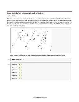
Modal Analysis for 3 pendulum with springs problem by Nasser M Abbasi This small note shows how to use Mathematica to solve symbolically for a problem in vibration to find the natural frequencies that a system of 3 masses will vibrate in. This digram below describes the problem. We use Lagrangian formulation to determine the equation of motions, then use modal analysis to decouple the system and solve it. In this system , the springs are attached at a distant a From the edge. Each pendulum has length L and has masses m1,m2,m3 attached to the end. The initial conditions are q (0)={Pi/4,Pi/4,Pi/4} and q = { 0 , 0 , 0 } Define a function which accepts the kinetic and potential energy and return back the stiffness and the mass matrix In[1]:= Needs @ " Notation` " D In[2]:= Symbolize B q 1 F ; Symbolize B q 2 F ; Symbolize B q 3 F ; Symbolize B r 1 F ; Symbolize B r 2 F ; Symbolize B r 3 F ; Printed by Mathematica for Students In[8]:= obtainStiffnessAndMassMatrix @ ke_ , u_ D : = Module A 8 lagrangian , eq1 , eq2 , eq3 , meq1 , meq2 , meq3 , seq1 , seq2 , seq3 , stiffnessMatrix , massMatrix , any , lagrangian = ke - u ; eq1 = D @ D @ lagrangian , q 1 ' @ t D D , t D - D @ lagrangian , q 1 @ t D D Š 0 ; eq2 = D @ D @ lagrangian , q 2 ' @ t D D , t D - D @ lagrangian , q 2 @ t D D Š 0 ; eq3 = D @ D @ lagrangian , q 3 ' @ t D D , t D - D @ l
2 agrangian , q 3 @ t D D Š 0 ; H * l
agrangian , q 3 @ t D D Š 0 ; H * linearize using small angle approximation * L eq1 = eq1 . Sin @ q 1 @ t D D �- q 1 @ t D ; eq2 = eq2 . Sin @ q 2 @ t D D �- q 2 @ t D ; eq3 = eq3 . Sin @ q 3 @ t D D �- q 3 @ t D ; Print @ " Equation of motion are " D ; Print @ 8 eq1 , eq2 , eq3 TableForm D ; seq1 = eq1 . q 1 ¢¢ @ t D _ ® 0 ; seq2 = eq2 . q 2 ¢¢ @ t D _ ® 0 ; seq3 = eq3 . q 3 ¢¢ @ t D _ ® 0 ; z1 = eq1 . any_ == 0 ® any ; z2 = seq1 . any_ Š 0 ® any ; meq1 = I eq1 . any_ == 0 ® any M - I seq1 . any_ Š 0 ® any M Simplify ; z1 = eq2 . any_ == 0 ® any ; z2 = seq2 . any_ Š 0 ® any ; meq2 = H z1 - z2 L FullSimplify ; meq3 = I eq3 . any_ == 0 ® any M - I seq3 . any_ Š 0 ® any M Simplify ; r = Normal @ CoefficientArrays @ 8 seq1 , seq2 , seq3 , 8 q 1 @ t D , q 2 @ t D , q 3 @ t D D D ; stiffnessMatrix = Collect @ r @ @ 2 , All D D , a D ; r = Normal @ CoefficientArrays @ 8 meq1 , meq2 , meq3 , 8 q 1 '' @ t D , q 2 '' @ t D , q 3 '' @ t D D D ; massMatrix = Collect @ r @ @ 2 , All D D , a D ; 8 massMatrix , stiffnessMatrix E Now define the kinetic and potenatial energy In[9]:= ke = 1 2 m 1 H L q 1 ' @ t D L 2 + 1 2 m 2 H L q 2 ' @ t D L 2 + 1 2 m 3 H L q 3 ' @ t D L 2 ; u = 1 2 k 1 H a q 2 @ t D - a q 1 @ t D L 2 + 1 2 k 2 H a q 3 @ t D - a q 2 @ t D L 2
3 + m 1 g L H 1 - Cos @ q 1 @ t D D L + m
+ m 1 g L H 1 - Cos @ q 1 @ t D D L + m 2 g L H 1 - Cos @ q 2 @ t D D L + m 3 g L H 1 - Cos @ q 3 @ t D D L ; Now call the above function to generate the stiffness and mass matrix. It also prints the 3 equations of motion In[11]:= 8 massMatrix , stiffnessMatrix = obtainStiffnessAndMassMatrix @ ke , u D ; 2 note1.nb Printed by Mathematica for Students Equation of motion are g L m 1 q 1 @ t D - a k 1 H - a q 1 @ t D + a q 2 @ t D L + L 2 m 1 H q 1 L ¢¢ @ t D Š 0 g L m 2 q 2 @ t D + a k 1 H - a q 1 @ t D + a q 2 @ t D L - a k 2 H - a q 2 @ t D + a q 3 @ t D L + L 2 m 2 H q 2 L ¢¢ @ t D Š 0 g L m 3 q 3 @ t D + a k 2 H - a q 2 @ t D + a q 3 @ t D L + L 2 m 3 H q 3 L ¢¢ @ t D Š 0 Now print the STIFFNESS and MASS matrix In[12]:= vars = 8 q 1 '' @ t D , q 2 '' @ t D , q 3 '' @ t D ; deps = 8 q 1 @ t D , q 2 @ t D , q 3 @ t D ; Print @ MatrixForm @ massMatrix D , MatrixForm @ Transpose @ List @ vars D D D , " + " , MatrixForm @ stiffnessMatrix D , MatrixForm @ Transpose @ List @ deps D D D D ; L 2 m 1 0 0 0 L 2 m 2 0 0 0 L 2 m 3 H q 1 L ¢¢ @ t D H q 2 L ¢¢ @ t D H q 3 L ¢¢ @ t D + a 2 k 1 + g L m 1 - a 2 k 1 0 - a 2 k 1 a 2 H k 1 + k 2 L + g L m 2 - a 2 k 2 0 - a 2 k 2 a 2 k 2 + g L m 3 q 1 @ t D q 2 @ t D q 3 @ t D Now that we have the stiffness and mass matrix, we can perform modal analysis. Start by doing the first transformation In[16]:= invMassMatrix = MatrixPower B massMatrix , - 1 2 F ;
4 Print @ " new K matrix = " , MatrixForm
Print @ " new K matrix = " , MatrixForm @ newK = invMassMatrix . stiffnessMatrix . invMassMatrix D D ; new K matrix = a 2 k 1 + g L m 1 L 2 m 1 - a 2 k 1 L 2 m 1 L 2 m 2 0 - a 2 k 1 L 2 m 1 L 2 m 2 a 2 H k 1 + k 2 L + g L m 2 L 2 m 2 - a 2 k 2 L 2 m 2 L 2 m 3 0 - a 2 k 2 L 2 m 2 L 2 m 3 a 2 k 2 + g L m 3 L 2 m 3 In[20]:= values = 8 m 1 ® 1 , m 2 ® 2 , m 3 ® 3 , k 1 ® 10 , L ® 1 , a ® .5 , k 2 ® 2 , g ® 9.8 ; invMassMatrix = invMassMatrix . values ; massMatrix = massMatrix . values ; newK = newK . values Out[23]= 8 8 12.3 , - 1.76777 , 0 , 8 - 1.76777 , 11.3 , - 0.204124 , 8 0 , - 0.204124 , 9.96667 In[24]:= 8 lambda , eigvect = Eigensystem @ newK D ; Print @ " Eigenvalues = " , lambda D ; Eigenvalues = 8 13.6413 , 10.1254 , 9.8 In[26]:= eigvect = Transpose @ eigvect D ; eigvect = eigvect Map @ Norm , eigvect D ; Print @ " Eigenvectors = " , eigvect D ; Eigenvectors = 8 8 0.796202 , - 0.446538 , 0.408248 , 8 - 0.6041 , - 0.5493 , 0.57735 , 8 0.0335579 , 0.70631 , 0.707107 Now find L matrix note1.nb 3 Printed by Mathematica for Students Now find L matrix In[29]:= L = Transpose @ eigvect D . newK . eigvect Chop Out[29]= 8 8 13.6413 , 0 , 0 , 8 0 , 10.1254 , 0 , 8 0 , 0 , 9.8 Hence the decoupled system of differential equations is In[30]:= vars = 8 r 1 '' @ t D , r 2 '' @ t D , r 3 '' @ t D ; deps = 8 r 1 @ t D , r 2 @ t D , r 3 @ t D ; Print @ MatrixForm @ Transpose @ List @ vars D
5 D D , " + " , MatrixForm @ L D , Matrix
D D , " + " , MatrixForm @ L D , MatrixForm @ Transpose @ List @ deps D D D D ; H r 1 L ¢¢ @ t D H r 2 L ¢¢ @ t D H r 3 L ¢¢ @ t D + 13.6413 0 0 0 10.1254 0 0 0 9.8 r 1 @ t D r 2 @ t D r 3 @ t D Now convert the IC from q (t) space to r (t) space In[35]:= initial q = 8 Pi 4 , Pi 2 , Pi 4 ; initialR = Transpose @ eigvect D . MatrixPower B massMatrix , 1 2 F . initial q Chop Out[36]= 8 - 0.670986 , - 0.610119 , 2.5651 In[37]:= initial q Dot = 8 0 , 0 , 0 ; initialRDot = Transpose @ eigvect D . MatrixPower B massMatrix , 1 2 F . initial q Dot Out[38]= 8 0. , 0. , 0. Now solve the r (t) system In[42]:= eq = r 1 '' @ t D + L @ @ 1 , 1 D D r 1 @ t D Š 0 ; solr1 = First @ DSolve @ 8 eq , r 1 @ 0 D == initialR @ @ 1 D D , r 1 ' @ 0 D == initialRDot @ @ 1 D D , r 1 @ t D , t D D ; Print @ " r 1 @ t D = " , solr1 = r 1 @ t D . solr1 D r 1 @ t D = - 0.670986 Cos @ 3.69341 t D In[45]:= eq = r 2 '' @ t D + L @ @ 2 , 2 D D r 2 @ t D Š 0 ; solr2 = First @ DSolve @ 8 eq , r 2 @ 0 D == initialR @ @ 2 D D , r 2 ' @ 0 D == initialRDot @ @ 2 D D , r 2 @ t D , t D D ; Print @ " r 2 @ t D = " , solr2 = r 2 @ t D . solr2 D r 2 @ t D = - 0.610119 Cos @ 3.18205 t D 4 note1.nb Printed by Mathematica for Students In[48]:= eq = r 3 '' @ t D + L @ @ 3 , 3 D D r 3 @ t D Š 0 ; solr3 = First @ DSolve @ 8 eq , r 3 @ 0 D == initialR @ @ 3 D D , r 3 ' @ 0 D == initialRDot @ @ 3 D D , r 3 @ t D , t D D
6 ; Print @ " r 3 @ t D = " , solr3 = r 3
; Print @ " r 3 @ t D = " , solr3 = r 3 @ t D . solr3 D r 3 @ t D = 2.5651 Cos @ 3.1305 t D Now convert solution from r (t) to q (t) In[51]:= MatrixForm @ sol q = invMassMatrix . eigvect . 8 8 solr1 , 8 solr2 , 8 solr3 D Out[51]//MatrixForm= 1.0472 Cos @ 3.1305 t D + 0.272441 Cos @ 3.18205 t D - 0.53424 Cos @ 3.69341 t D 1.0472 Cos @ 3.1305 t D + 0.236978 Cos @ 3.18205 t D + 0.28662 Cos @ 3.69341 t D 1.0472 Cos @ 3.1305 t D - 0.248799 Cos @ 3.18205 t D - 0.0130001 Cos @ 3.69341 t D In[52]:= sol q 1 = sol q @ @ 1 D D ; sol q 2 = sol q @ @ 2 D D ; sol q 3 = sol q @ @ 3 D D ; Now plot the solutions In[55]:= Print @ " q 1 @ t D = " , sol q 1 = First @ Simplify @ Chop @ ExpToTrig @ sol q 1 . values D D D D D ; q 1 @ t D = 1.0472 Cos @ 3.1305 t D + 0.272441 Cos @ 3.18205 t D - 0.53424 Cos @ 3.69341 t D In[56]:= Print @ " q 2 @ t D = " , sol q 2 = First @ FullSimplify @ Chop @ ExpToTrig @ sol q 2 . values D D D D D ; q 2 @ t D = 1.0472 Cos @ 3.1305 t D + 0.236978 Cos @ 3.18205 t D + 0.28662 Cos @ 3.69341 t D In[57]:= Print @ " q 3 @ t D = " , sol q 3 = First @ Simplify @ Chop @ ExpToTrig @ sol q 3 . values D D D D D ; q 3 @ t D = 1.0472 Cos @ 3.1305 t D - 0.248799 Cos @ 3.18205 t D - 0.0130001 Cos @ 3.69341 t D note1.nb 5 Printed by Mathematica for Students In[58]:= Plot @ 8 sol q 1 , sol q 2 , sol q 3 , 8 t , 0 , 10 D Out[58]= 2 4 6 8 10 - 1.5 - 1.0 - 0.5 0.5 1.0 1.5 6 note1.nb Printed by Mathematica for Stude