Probability Basics CS771: Introduction to Machine Learning - PowerPoint Presentation

1. Probability BasicsCS771: Introduction to Machine LearningNisheeth

2. Random Variables2Informally, a random variable (r.v.) denotes possible outcomes of an eventCan be discrete (i.e., finite many possible outcomes) or continuousSome examples of discrete r.v.denoting outcomes of a coin-tossdenoting outcome of a dice rollSome examples of continuous r.v.denoting the bias of a coindenoting heights of students in CS771denoting time to get to your hall from the department   (a discrete r.v.) (a continuous r.v.) 

3. Discrete Random Variables3For a discrete r.v. , denotes - probability that is called the probability mass function (PMF) of r.v. or is the value of the PMF at     

4. Continuous Random Variables4For a continuous r.v. , a probability or is meaninglessFor cont. r.v., we talk in terms of prob. within an interval is the prob. that as is the probability density at   

5. Discrete example: roll of a diexp(x)1/6145623

6. Probability mass function (pmf)xp(x)1p(x=1)=1/62p(x=2)=1/63p(x=3)=1/64p(x=4)=1/65p(x=5)=1/66p(x=6)=1/6

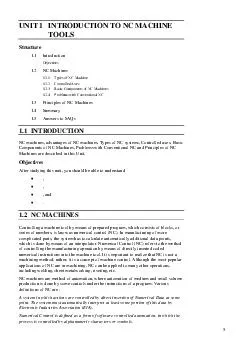
7. Cumulative distribution functionxP(x≤A)1P(x≤1)=1/62P(x≤2)=2/63P(x≤3)=3/64P(x≤4)=4/65P(x≤5)=5/66P(x≤6)=6/6

8. Cumulative distribution function (CDF)xP(x)1/61456231/31/22/35/61.0

9. Practice ProblemThe number of patients seen in a clinic in any given hour is a random variable represented by x. The probability distribution for x is:x1011121314P(x).4.2.2.1.1Find the probability that in a given hour:a.    exactly 14 patients arriveb.    At least 12 patients arrivec.    At most 11 patients arrive  p(x=14)= .1 p(x12)= (.2 + .1 +.1) = .4 p(x≤11)= (.4 +.2) = .6

10. Continuous case The probability function that accompanies a continuous random variable is a continuous mathematical function that integrates to 1. For example, recall the negative exponential function (in probability, this is called an “exponential distribution”): This function integrates to 1:

11. Continuous case: “probability density function” (pdf)xp(x)=e-x1The probability that x is any exact particular value (such as 1.9976) is 0; we can only assign probabilities to possible ranges of x.

12. For example, the probability of x falling within 1 to 2:xp(x)=e-x112

13. Example 2: Uniform distributionThe uniform distribution: all values are equally likely.f(x)= 1 , for 1 x 0 xp(x)11We can see it’s a probability distribution because it integrates to 1 (the area under the curve is 1): 

14. Example: Uniform distribution What’s the probability that x is between 0 and ½? P(½ x 0)= ½ xp(x)11½0

15. A word about notation15can mean different things depending on the context denotes the distribution (PMF/PDF) of an r.v. or or simply denotes the prob. or prob. density at value Actual meaning should be clear from the context (but be careful)Exercise same care when is a specific distribution (Bernoulli, Gaussian, etc.)The following means generating a random sample from the distribution   

16. Joint Probability Distribution16Joint prob. dist. models probability of co-occurrence of two r.v. For discrete r.v., the joint PMF is like a table (that sums to 1)For two continuous r.v.’s and , we have joint PDF  For 3 r.v.’s, we will likewise have a “cube” for the PMF. For more than 3 r.v.’s too, similar analogy holds For more than two r.v.’s, we will likewise have a multi-dim integral for this property

17. Marginal Probability Distribution17Consider two r.v.’s X and Y (discrete/continuous – both need not of same type)Marg. Prob. is PMF/PDF of one r.v. accounting for all possibilities of the other r.v.For discrete r.v.’s, and For discrete r.v. it is the sum of the PMF table along the rows/columnsFor continuous r.v.’s,  The definition also applied for two sets of r.v.’s and marginal of one set of r.v.’s is obtained by summing over all possibilities of the second set of r.v.’sFor discrete r.v.’s, marginalization is called summing over, for continuous r.v.’s, it is called “integrating out”

18. Conditional Probability Distribution18Consider two r.v.’s and (discrete/continuous – both need not of same type)Conditional PMF/PDF is the prob. dist. of one r.v. , fixing other r.v. or like taking a slice of the joint dist. Note: A conditional PMF/PDF may also be conditioned on something that is not the value of an r.v. but some fixed quantity in general Discrete Random VariablesContinuous Random VariablesWe will see cond. dist. of output given weights (r.v.) and features written as  

19. An exampleX/YrainingsunnyUmbrella0.50.1No umbrella0.20.2P(x) = {0.6, 0.4}P(y) = {0.7, 0.3}P(X|Y = raining) = {0.5, 0.2}P(X = umbrella|Y = raining)ABP (B|A)p(A) = p(A|B)p(B) P(A,B)

20. Some Basic Rules20Sum Rule: Gives the marginal probability distribution from joint probability distributionProduct Rule: Bayes’ rule: Gives conditional probability distribution (can derive it from product rule)Chain Rule:  

21. Independence21 and are independent when knowing one tells nothing about the otherThe above is the marginal independence Two r.v.’s and may not be marginally indep but may be given the value of another r.v.  

22. Expectation22Expectation of a random variable tells the expected or average value it takesExpectation of a discrete random variable having PMF Expectation of a continuous random variable having PDF The definition applies to functions of r.v. too (e.g.., )Exp. is always w.r.t. the prob. dist. of the r.v. and often written as    Often the subscript is omitted but do keep in mind the underlying distributionNote that this exp. is w.r.t. the distribution of the r.v.   Probability that  Probability density at  

23. Expectation: A Few Rules23Expectation of sum of two r.v.’s: Proof is as followsDefine s.t. where and   and need not be even independent. Can be discrete or continuous Used the rule of marginalization of joint dist. of two r.v.’s

24. Expectation: A Few Rules (Contd)24Expectation of a scaled r.v.: Linearity of expectation: (More General) Lin. of exp.: Exp. of product of two independent r.v.’s: Law of the Unconscious Statistician (LOTUS): Given an r.v. with a known prob. dist. and another random variable for some function Rule of iterated expectation: ]  and are arbitrary functions.    Requires finding  Requires only which we already have LOTUS also applicable for continuous r.v.’sand are real-valued scalars is a real-valued scalar 

25. Variance and Covariance25Variance of a scalar r.v. tells us about its spread around its mean value Standard deviation is simply the square root is varianceFor two scalar r.v.’s and , the covariance is defined byFor two vector r.v.’s and (assume column vec), the covariance matrix is defined byCov. of components of a vector r.v. : Note: The definitions apply to functions of r.v. too (e.g., Note: Variance of sum of independent r.v.’s:     Important result

26. Transformation of Random Variables26Suppose be a linear function of a vector-valued r.v. ( is a matrix and is a vector, both constants)Suppose and , then for the vector-valued r.v. Likewise, if be a linear function of a vector-valued r.v. ( is a vector and is a scalar, both constants)Suppose and , then for the scalar-valued r.v.      

27. Common Probability Distributions27Important: We will use these extensively to model data as well as parameters of modelsSome common discrete distributions and what they can modelBernoulli: Binary numbers, e.g., outcome (head/tail, 0/1) of a coin tossBinomial: Bounded non-negative integers, e.g., # of heads in coin tossesMultinomial/multinoulli: One of (>2) possibilities, e.g., outcome of a dice rollPoisson: Non-negative integers, e.g., # of words in a documentSome common continuous distributions and what they can modelUniform: numbers defined over a fixed rangeBeta: numbers between 0 and 1, e.g., probability of head for a biased coinGamma: Positive unbounded real numbersDirichlet: vectors that sum of 1 (fraction of data points in different clusters)Gaussian: real-valued numbers or real-valued vectors