PPT-Bioinformatics III 1 V23 Integrated Metabolic and Transcriptional Networks

Author : naomi | Published Date : 2024-03-13

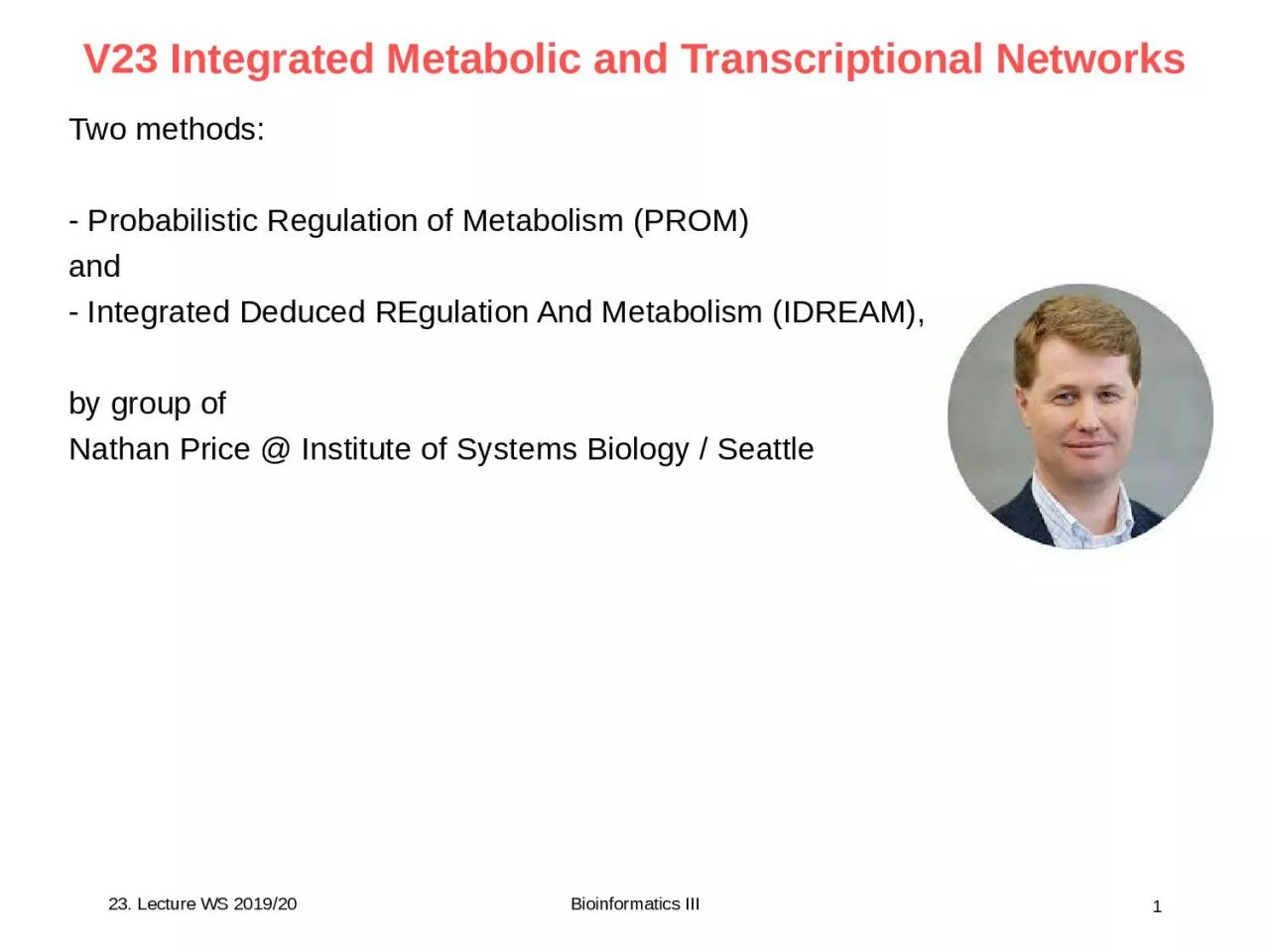
Two methods Probabilistic Regulation of Metabolism PROM and Integrated Deduced REgulation And Metabolism IDREAM by group of Nathan Price Institute

Presentation Embed Code

Download Presentation

Download Presentation The PPT/PDF document "Bioinformatics III 1 V23 Integrated Meta..." is the property of its rightful owner. Permission is granted to download and print the materials on this website for personal, non-commercial use only, and to display it on your personal computer provided you do not modify the materials and that you retain all copyright notices contained in the materials. By downloading content from our website, you accept the terms of this agreement.

Bioinformatics III 1 V23 Integrated Metabolic and Transcriptional Networks: Transcript

Two methods Probabilistic Regulation of Metabolism PROM and Integrated Deduced REgulation And Metabolism IDREAM by group of Nathan Price Institute of. Jesse Gray. Neurobiology department. Harvard Medical School. Animals store life-long memories. Neuronal circuits are rewired by experience according to genomic instructions. Experience…. rewires circuits…. Borodovsky. . a short intro . Position open:. . Scientist - Pathway Informatics (June 2009). THE POSITION . The successful candidate will join the Computational Science & Bioinformatics team. Data . and Analysis . Tools for . Herpesviridae. Viruses . in . the Virus Pathogen Resource (. ViPR. ). Yun Zhang. 1. , Brett Pickett. 1. , Eva . Sadat. 2. , . , R. Burke . Squires. 2. , . Jyothi. Noronha. Chemostat. Cultures of . Saccharomyces . cerevisiae. . Subjected to Diurnal Temperature Cycle. Kevin Wyllie and Monica Hong. 05/27/15. Hebly. , M. (2014). Physiological and Transcriptional Responses of Anaerobic . GEP Alumni Consortium. NSF Improving Undergraduate STEM Education Grants. Effective Implementation of a Classroom Undergraduate Research Experience (CURE): Testing, Optimizing, and Extending a Bioinformatics Approach. – where are we in 2011?. What I aim to do in 30 minutes.... . Give you a brief intro into our system of study.. . Recap the things we talked about in York in York in 2009.. Think about what we could do in Edinburgh in 2011. Chemostat. Cultures of . Saccharomyces . cerevisiae. . Subjected to Diurnal Temperature Cycle. Kevin Wyllie and Monica Hong. 05/27/15. Hebly. , M. (2014). Physiological and Transcriptional Responses of Anaerobic . A. W. Schreiber. Australian Centre for Plant Functional Genomics. Waite Campus, . University of Adelaide. Achievements and new directions. in Subatomic Physics:. Workshop in Honour of Tony . Thomas’s 60. High-throughput Data Analysis. Literature Study. Data Mining . Functional Genomics Analysis. Vector NTI Advance®. Software. License type. License number. 2008. 2009. 2010. 2011. 2012. 2013. 2014. Galaxy. Section 1: Introduction and biological databases.. Section 2: Sequence alignment.. Section 3: Gene and promoter prediction.. Section 4: Molecular phylogenetics.. Section 5: Structural Bioinformatics. Intermediary Metabolism. OR. Interrelationship Between Various Metabolic . Pathways. OR. Interdependence Of Metabolic Pathways. To Better Understand Metabolism Of Various Biomolecules . Metabolism of each . Aedes aegypti. David Price. Disease Vector Molecular Biology Lab. NMSU. PI . Immo. Hansen. Background. Aedes aegypti . is an important disease vector. Relatively safe model for malaria. Plasmodium . Karsten Hokamp, PhD. TCD Bioinformatics Support Team. TCD, 26/08/2015. Overview. Programming. First Python script/program. Why . Python. ?. Bioinformatics examples. Additional resources. Outlook. What is programming and why bother?. There exist different levels of computational methods for . describing metabolic networks:. - stoichiometry/kinetics of classical biochemical . pathways. (glycolysis, TCA cycle, .... - stoichiometric modelling (.

Download Document

Here is the link to download the presentation.
"Bioinformatics III 1 V23 Integrated Metabolic and Transcriptional Networks"The content belongs to its owner. You may download and print it for personal use, without modification, and keep all copyright notices. By downloading, you agree to these terms.