
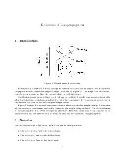
are just Backprop Jason Eisner tutorial paper The insideoutside algorithm is the hardest algorithm I know a senior NLP researcher ID: 663547
Download Presentation The PPT/PDF document "1 Inside-Outside & Forward-Backw..." is the property of its rightful owner. Permission is granted to download and print the materials on this web site for personal, non-commercial use only, and to display it on your personal computer provided you do not modify the materials and that you retain all copyright notices contained in the materials. By downloading content from our website, you accept the terms of this agreement.


Slide1
1
Inside-Outside & Forward-Backward Algorithms are just Backprop
Jason Eisner
(tutorial paper)Slide2
“The inside-outside algorithm is the hardest algorithm I know.” – a senior NLP researcher, in the 1990’sWhat does inside-outside do?It computes expected counts of substructures ...… that appear in the true parse of some sentence w. 2
Slide3
Where are the constituents?3
coal
energy
expert
witness
p=0.5Slide4
Where are the constituents?4
coal
energy
expert
witness
p=0.1Slide5
Where are the constituents?5
coal
energy
expert
witness
p=0.1Slide6
Where are the constituents?6
coal
energy
expert
witness
p=0.1Slide7
Where are the constituents?7
coal
energy
expert
witness
p=0.2Slide8
Where are the constituents?8
coal
energy
expert
witness
0.5
+0.1
+0.1
+0.1
+0.2
= 1Slide9
flieslikeanTimearrow
Where are NPs, VPs, … ?
9
flies
like
an
Time
arrow
NP locations
VP locations
VP
NP
NP
PP
S
V
P
Det
NSlide10
Where are NPs, VPs, … ?10
flies
like
an
Time
arrow
flies
like
an
Time
arrow
NP locations
VP locations
p=0.5
(S (NP Time) (VP flies (PP like (NP an arrow))))Slide11
Where are NPs, VPs, … ?11
flies
like
an
Time
arrow
flies
like
an
Time
arrow
NP locations
VP locations
p=0.3
(S (NP Time flies) (VP like (NP an arrow)))Slide12
Where are NPs, VPs, … ?12
flies
like
an
Time
arrow
flies
like
an
Time
arrow
NP locations
VP locations
p=0.1
(S (VP Time (NP (NP flies) (PP like (NP an arrow)))))Slide13
Where are NPs, VPs, … ?13
flies
like
an
Time
arrow
flies
like
an
Time
arrow
NP locations
VP locations
p=0.1
(S (VP (VP Time (NP flies)) (PP like (NP an arrow))))Slide14
Where are NPs, VPs, … ?14
flies
like
an
Time
arrow
NP locations
flies
like
an
Time
arrow
VP locations
0.5
+0.3
+0.1
+0.1
= 1Slide15
How many NPs, VPs, … in all?15
flies
like
an
Time
arrow
NP locations
flies
like
an
Time
arrow
VP locations
0.5
+0.3
+0.1
+0.1
= 1Slide16
How many NPs, VPs, … in all?16flies
likean
Timearrow
NP locations
flieslike
anTime
arrow
VP locations
2.1 NPs
(expected)
1.1 VPs
(expected)Slide17
Where did the rules apply?17
flies
like
an
Time
arrow
flies
like
an
Time
arrow
S
NP VP locations
NP
Det
N locationsSlide18
Where did the rules apply?18
flies
like
an
Time
arrow
flies
like
an
Time
arrow
S
NP VP locations
NP
Det
N locations
p=0.5
(S (NP Time) (VP flies (PP like (NP an arrow))))Slide19
Where is S NP VP substructure?19
flies
like
an
Time
arrow
flies
like
an
Time
arrow
S
NP VP locations
NP
Det
N locations
p=0.3
(S (NP Time flies) (VP like (NP an arrow)))Slide20
Where is S NP VP substructure?20
flies
like
an
Time
arrow
flies
like
an
Time
arrow
S
NP VP locations
NP
Det
N locations
p=0.1
(S (VP Time (NP (NP flies) (PP like (NP an arrow)))))Slide21
Where is S NP VP substructure?21
flies
like
an
Time
arrow
flies
like
an
Time
arrow
S
NP VP locations
NP
Det
N locations
p=0.1
(S (VP (VP Time (NP flies)) (PP like (NP an arrow))))Slide22
Why do we want this info?Grammar reestimation by EM methodE step collects those expected countsM step setsMinimum Bayes Risk decodingFind a tree that maximizes expected reward,e.g., expected total # of correct constituentsCKY-like dynamic programming algorithm The input specifies the probability of correctness for each possible constituent (e.g., VP from 1 to 5)22Slide23
Why do we want this info?Soft features of a sentence for other tasksNER system asks: “Is there an NP from 0 to 2?”True answer is 1 (true) or 0 (false)But we return 0.3, averaging over all parsesThat’s a perfectly good feature value – can be fed as to a CRF or a neural network as an input featureWriting tutor system asks: “How many times did the student use S NP[singular] VP[plural]?”True answer is in {0, 1, 2, …}But we return 1.8, averaging over all parses23Slide24
How do we compute it all?How I usually teach it:24CKY recognizerinside algorithminside-outside algorithm
develop an analogy
to forward-backward
add weights
But algorithm is confusing, and I wave
my hands instead of giving a real proof
historically
accurateSlide25
600.465 - Intro to NLP - J. Eisner
25
VP
(1,5) =
p(
flies like an arrow |
VP
)
VP
(1,5) =
p(
time VP today |
S)
Inside & Outside Probabilities
S
NP
time
VP
VP
NP
today
V
flies
PP
P
like
NP
Det
an
N
arrow
VP
(1,5)
*
VP
(1,5)
= p(
time [VP
flies like an arrow
] today
|
S)
“inside” the VP
“outside” the VPSlide26
600.465 - Intro to NLP - J. Eisner
26
VP
(1,5) =
p(
flies like an arrow |
VP
)
VP
(1,5) =
p(
time VP today |
S)
Inside & Outside Probabilities
S
NP
time
VP
VP
NP
today
V
flies
PP
P
like
NP
Det
an
N
arrow
VP
(1,5)
*
VP
(1,5)
=
p(
time
flies like an arrow
today
&
VP
(1,5)
| S)
/
S
(0,6)
p(time flies like an arrow today | S)
= p(
VP
(1,5)
| time flies like an arrow today, S)Slide27
600.465 - Intro to NLP - J. Eisner
27
VP
(1,5) =
p(
flies like an arrow |
VP
)
VP
(1,5) =
p(
time VP today |
S)
Inside & Outside Probabilities
S
NP
time
VP
VP
NP
today
V
flies
PP
P
like
NP
Det
an
N
arrow
So
VP
(1,5)
*
VP
(1,5)
/
s
(0,6)
is probability that there is a VP here,
given all of the observed data (words)
analogous
to forward-backward
in the finite-state case!
Start
C
H
C
H
C
HSlide28
How do we compute it all?How I usually teach it:28CKY recognizerinside algorithminside-outside algorithm
develop an analogy
to forward-backward
add weights
But algorithm is confusing, and I wave
my hands instead of giving a real proof
historically
accurate
This step
for free
as
backprop!Slide29
Back-Propagation29arithmetic circuit(computation graph)Slide30
Energy-Based ModelsDefineThenLog-linear case: 30Slide31
p(tree T | sentence w) is log-linear31Therefore, ∇ log Z will give expected rule counts.
total
prob
of all parsesSlide32
∇log Z = Expected Counts32Optimization
Gradient
Expected counts
novel alg
.Slide33
∇log Z = Expected Counts33OptimizationGradient
Expected counts
backprop
(EM) & MBR decoding & soft features
Not only does this
get the same answer,
it actually gives the
identical algorithm!Slide34
TerminologyAutomatic differentiation: Given a circuit that computes a function f, construct a circuit to compute (f, ∇f)34Slide35
TerminologyAutomatic differentiation: Given a circuit that computes a function f, construct a circuit to compute (f, ∇f)Algorithmic differentiation:Given code that computes a function f, construct code to compute (f, ∇f)Back-propagation:One computational strategy that the new circuit or code can use35Slide36
Inside algorithm computes ZEssentially creates a circuit “on the fly” Like other dynamic programming algorithmsCircuit structure gives parse forest hypergraphO(Vn2) nodes in the circuit, with names like (VP,1,5)Each node sums O(V2n) 3-way productsThe 3-way products and the intermediate sums aren’t nodes of the formal circuitNo names, not stored long-term36Slide37
Inside algorithm computes Z37
visit nodesbottom-up
(toposort)Slide38
How to differentiate38
(“swap” x, y
1
)
(“swap” x, y
2
)Slide39
Inside algorithm has 3-way products39
(swap A, G)
(swap A, B)
(swap A, C)
(A += G*B*C)Slide40
Inside algorithm has 3-way products40
ð
[…]
is traditionally
called […]
We’ll similarly write
ð
G
[A
B C
] as [A
B C
]Slide41
Differentiate to compute (Z, ∇Z)41
visit ð nodesin reverse
order of
(so top-down)wait, what’s this line?Slide42
The final step: / Z42
could reasonably
rename G(R) to
(R)
we want this
but oops, we used backprop
to get this,
so fix itSlide43
The final step: / ZThis final step is annoying. It’s more chain rule. Shouldn’t that be part of backprop? We won’t need it if we actually compute ∇ log Z in the first place (straightforwardly).We only did ∇Z for pedagogical reasons.It’s closer to the original inside-outside algorithm, and ensures ð = traditional .But the “straightforward” way is slightly more efficient.43Slide44
Inside algorithm has 3-way products44
ð
[…]
is traditionally
called […]
Paper spells out why the traditional “outer weight” interpretation of
is actually a partial derivativeSlide45
Other algorithms! E.g.:45FormalismHow to compute Z(total weight of all derivations)Expected counts of substructures = ∇log ZHMM
backward algorithmbackpropPCFG in CNFinside algorithmbackprop
CRF-CFG in CNF
inside algorithmbackpropsemi-Markov CRFSaragawi & Cohen 2004
backproparbitrary PCFGEarley’s algorithmbackprop
CCGVijay-Shankar & Weir 1990backprop
TAG
Vijay-Shankar & Joshi 1987
backprop
dependency grammar
Eisner
&
Satta
backprop
transition-based parsing
PDA
with graph-structured stack
backprop
synchronous grammar
synchronous inside
algorithm
backprop
graphical model
junction tree
backpropSlide46
Other tips in the paperAn inside-outside algorithm should only be a few times as slow as its inside algorithm.People sometimes publish algorithms that are n times slower. This is a good reason to formally go through algorithmic differentiation.46Slide47
Other tips in the paperAn inside-outside algorithm should only be a few times as slow as its inside algorithm.HMMs can be treated as a special case of PCFGs.47Slide48
Other tips in the paperAn inside-outside algorithm should only be a few times as slow as its inside algorithm.HMMs can be treated as a special case of PCFGs.There are 2 other nice derivations of inside-outside. All yield essentially the same code, and the other perspectives are useful too.The Viterbi variant is useful for pruning (max-marginal counts) and parsing (Viterbi outside scores). It can be obtained as the 0-temperature limit of the gradient-based algorithm.The gradient view makes it easy to do end-to-end training if the parser talks to / listens to neural nets.48