
Outline Contour drawing in art S il h o uette outline Definition of outlines Image space Object space Image space methods Edge detection First order methods Second order methods Edge ID: 815424
Download The PPT/PDF document "Contour drawing / Edge detection" is the property of its rightful owner. Permission is granted to download and print the materials on this web site for personal, non-commercial use only, and to display it on your personal computer provided you do not modify the materials and that you retain all copyright notices contained in the materials. By downloading content from our website, you accept the terms of this agreement.


Slide1
Contour drawing / Edge detection
Slide2Outline
Contour drawing in art
S
il
h
o
uette
/ outline
Definition of outlines
Image space
Object space
Image space methods
Edge detection
First order methods
Second order methods
Edge
detection
using
non
color
buffers
Object space methods
Rendering object space contours
Occluding contours
Suggestive Contours
Ridges/valleys
Other GPU based methods
2pass drawing
Occluding edge extraction
Occluding contour detection in pixel
shader
Slide3Contour
drawing
in art
„The purpose of contour drawing is to emphasize the
mass
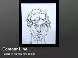
and volume of the subject rather than the detail; the focus is on the outlined shape of the subject and not the minor details.”https://en.wikipedia.org/wiki/Contour_drawingIn classic art several contour drawing techniques and exercises exist:
For computer graphics, contour drawing technique is the most revelant.It shows the main shape and edges of the scene omitting tone and fine geometric details. Compared to Blind/Timed drawings, contour drawings provide realistic representation of the subjects.
Blind Contour Drawing
Timed Drawing
Continuous Line Drawing
Contour drawing
Cross contour drawing
Etc..
Slide4Contour drawing in art
„The purpose of contour drawing is to emphasize the
mass
and
volume
of the subject rather than the detail; the focus is on the outlined shape of the subject and not the minor details.”https://en.wikipedia.org/wiki/Contour_drawingIn classic art several contour drawing techniques and exercises exist.
For details see:https://www.studentartguide.com/articles/line-drawings
Slide5Contour drawing
Works of David
Hockney
Sil
ho
uette
Object boundaries
Plane changes
Occlusion
Color change
Sharp edges
(
Ridges
/
valleys
)
Some features that can be expressed with contours
Slide6Abstract contour drawing
Many fine art contour drawings are not realistic but abstract
These are hard to reproduce with computer graphics
Recent solutions use neural networks and machine learning
Leon A.
Gatys, Alexander S. Ecker, Matthias Bethge: A Neural Algorithm of Artistic Style. Published in ArXiv 2015
Henri Matisse „...la torsem et native nue...” 1932
Slide7Definition of outlines in 3D graphics
Image space
Search for features on images
RGB image is always present
Additional images can be rendered:
DepthNormalObject IDEdge detection algorithms used in image processing and computer visionProCan be done in a post processOriginal geometry is not neededWe work on visible information only: occlusion is not a problem
ConLine stylization is harderTime coherency can be a problemHard to define „good” edges (false edges, missed edges)Sensible to noise
Object space
Search for features on the geometry (triangles)
Use vertex data: position and normal
Use topology data: triangle adjacency
Based on differential geometry
Pro
High quality can be achieved
Less false edges and edge misses
Line stylization is easier
Con
Occlusion can be a problem
Need geometry processing (deformable objects
can
not be preprocessed!)
Color change contours can not be handled
High quality lines need fine tessellation
Most contour extracting methods assume smooth geometry (no hard edges)
Slide8Image space methods
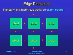
Detect edges on rendered images.
Edge: significant local change in image intensity.
Basic edge profile types (real edge can be a combination too):
Ramesh Jain,
Rangachar
Kasturi
, Brian G.
Schunck
: Machine Vision. Published by McGraw-Hill, Inc., ISBN 0-07-032018-7, 1995
http://www.cse.usf.edu/~r1k/MachineVisionBook/MachineVision.pdf
step
ramp
roof
line
Slide9Example
edge
profile
Slide10Slide11Edge detection
In computer vision contour detection usually has the following tasks:
Identify edge pixels on image
Try to form line segments or curve segments from distinct edge points
Merge segments into continuous contour lines
In NPR rendering we usually stop at the first step: find edge pixelsAnalyzing edge pixels, cleaning and merging them usually have too high costs
Slide12Finding edge pixels
Detect significant local changes: find local peaks in first derivative
Two example edge profiles in 1D:
F(x)
DF(x)
F(x)
DF(x)
OR
Edges are where the absolute value of the first derivative is
„
high enough
”
Slide13Finding edge pixels
Detect significant local changes: find local peaks in first derivative
Question:
R
endered image is 2D, what is the first gradient, and what is „high enough”?
Answer: Use partial derivatives:
Examine the magnitude of this vector
:
. Is it high enough?
In practice the sum of the absolute values of the partial derivatives can be used:
Slide14Finding edge pixels
Question:
R
endered image is vector valued (RGB), how to handle this?
Answer I.
Compute partial derivatives of color channels separately:
Examine this:
+
.
Or this:
+
Answer II.
Compute luminance of image -> scalar value image (prev. slide)
Some color contours could be missed!
Slide15How to calculate derivatives on image
Convolution matrix:
Problem: dx, and
dy
approximates the derivatives at different pixel positions ((x+0.5,y) and (x,y+0.5) respectively)
Slide16How to calculate derivatives on image
Roberts operator
Convolution matrix:
dx, and
dy
approximates the derivatives at the same pixel positions: (x+0.5, y+0.5), but not at (x, y)!
Slide17How to calculate derivatives on image
Central differences
Convolution matrix:
dx, and
dy
approximates the derivatives at (x, y), but discards pixel value at (x, y)!
Slide18How to calculate derivatives on image
Sobel operator
Convolution matrix:
Less sensible to noise.
Combination of a box blur and central differences.
One of the most commonly used differential operator
Slide19How to calculate derivatives on image
Prewitt operator
Convolution matrix:
Similar to Sobel, but closer pixels do not have higher influence.
Slide20Example
Grayscale image
Derivative in x direction
Derivative in y direction
Gradient magnitude
Slide21Example
RGB image
Gradient magnitude of R,G and B channels
Sum of gradient magnitudes
Threshold at 0.8 and invert
Threshold at 3.0 and invert
Slide22Comparison
Central Differences
Threshold = 0.3
Threshold = 0.9
The two methods are similar but Sobel has less noise e.g. here
Sobel
Slide23Threshold
Finding the right threshold value is hard
Depends on the image itself
Depends on the gradient operator
E
.g. in previous slide Sobel operator was normalized with a factor of 0.25 to match the central differences operatorIf low threshold is used, thick lines and noise will appearIf high threshold is used, important lines will disappear
Slide24Threshold problem
Function
Function derivative absolute value
Low threshold
High threshold
Too wide edge
Disappeared edge
A solution can be adaptive
thresholding
: adjust threshold value based on average gradient magnitude around the pixel
Con:
multipass
solution, needs preprocessing of gradient image
Slide25Higher order derivatives
First and second derivatives can be combined:
Keep zero crossings where
first derivative has high peak
(threshold again
, but edge width won’t grow as zero crossings positions can be calculated even at subpixel precision)
Function
First derivative
Edges at high (absolute) values
Second derivative
Edges at zero crossings
Slide26Second order derivative
Laplace operator
Divergence of the gradient
Convolution matrix
Or a smoothed version less sensible to noise:
Slide27Laplacian example I
Consider a pixel row:
First derivative:
Laplacian:
2
2
2
2
5
8
8
8
8
8
0
0
0
3
6
3
0
0
0
0
0
0
0
3
0
-3
0
0
0
0
Zero crossing with high first derivative
Zero crossings with low first derivative
Slide28Laplacian example II
Consider a pixel row:
First derivative:
Laplacian:
2
2
2
2
2
8
8
8
8
8
0
0
0
0
6
6
0
0
0
0
0
0
0
0
6
-6
0
0
0
0
Zero crossing is between pixels: harder to detect!
Laplacian works better on smooth edges.
Laplace operator is usually not used on its own, as second order derivatives are sensible to noise.
Now we have two good reasons to
prefilter
(blur) image before using Laplace operator!
Slide29Laplacian of Gaussian (LoG
)
Steps:
Smooth the image with Gaussian. (Can be a two pass separable filter.)
Apply Laplace operator.
Detect zero crossing with high first derivatives.Optional: edge location can even be estimated with subpixel resolution.
Gaussian
First
derivative
Second
Derivative
,
Laplacian
of Gaussian
(Mexican hat)
Slide30Laplacian of Gaussian result
We have three parameters that should be fine tuned:
Threshold for first derivative high peak
Threshold for zero crossing (if searching for pixels with near zero values, as an alternative more sophisticated zero crossing search can be used at higher cost)
Gaussian kernel width
Slide31Difference of Gaussians
(
DoG
)
Approximation of Laplacian of Gaussians
Use the difference of two Gaussian blursA Gaussian blur is a low pass filterA difference of two low pass filter is a band pass filter, just like the LaplacianThis is how the
retinal cells are believed to extract details
and
transfer
them
to
the
brain
Details
: Theory
of edge detection, D. Marr, E.
Hildreth, 1980. https://royalsocietypublishing.org/doi/pdf/10.1098/rspb.1980.0020More efficient implementation (Gaussians are separable)Steps:Smooth the image with Gaussian.
Smooth the image with Gaussian with different width.Compute difference of two smooth image.
Detect zero crossing on difference image.
Slide32Difference of Gaussians Result
Using wider Gaussians extracts main structures (lower frequency band is kept)
Using narrower Gaussians extracts fine details
(high
frequency band is kept)
XDoG
: advanced image stylization with
eXtended
Difference-of-Gaussians
, H.
Winnemöller
, NPAR11
Slide33Smooth
thresholding
:
XDoG
X
DoG: Advanced Image Stylization with E
xtended Difference-of-Gaussians. H. Winnemöller
NPAR
,
2011
.
XDoG
:
E
x
tended
D
ifference
-of-Gaussians
Idea: use a smoothstep function instead of a step
function for thresholdingEdges
are not binary
anymore, so the edge
map becomes softer
Slide34Smooth
thresholding
:
XDoG
DoG
Thresholding
with step
XDoG
Thresholding
with
smoothstep
Slide35Non color buffers
RGB image stores color information.
Edges appear at significant color differences.
Color difference can be caused by lighting and texture. These edges are not always wanted.
Object boundaries can have the same color: important edges will be lost.
We can use images storing non color information as the basis of edge detection:Camera space normalsCamera space depthObject ID (not always available in render engines)They can provide much cleaner edgesMethod: Calculate gradient for depth, normal, color, etc. maps separately and use the maximum or sum of these gradients for edge detection.
We have to find a good weighting for the separate gradients (normal gradients are probably in a smaller range than depth gradients)
Slide36Example
Depth based contours
Normal based contours
Combined depth and normal contours
Keep both features
Lost edges due to small depth difference
Lost edges due to same orientation of surfaces
Slide37Object space methods
Main workflow
Process triangle geometry
Extract polylines or curves describing the contours from the geometry
Send the lines through the graphics pipeline just like any other 3D objects
Lines can be rendered as line primitives orLines are converted to line strips/ribbons (in camera space to face the camera)Strips can be textured with artist given line textureTexture is typically semi-transparent (alpha blending)
Slide38How to extract contours from triangle geometry?
Contours are related to specific geometric features
Extracting contours
use
s
the theory of differential geometryVery basics:The first order approximation of a surface is its tangent plane, defined by its normal vector (normals = first order derivatives of the surface)The derivatives of normal vectors define second order features: curvature
R
R
R
N
N
N
Curvature = 1/R
Curvature at a point is the reciprocal of the radius of the circle that can tightly fit onto the curve at the given point.
Positive curvature
Positive curvature
Negative curvature
Slide39Curvatures and Principal curvatures
Curvature on a 3D surface is defined with respect to a direction in its tangent plane (normal curvature)
Two special directions exists
The direction where the surface has largest curvature
The direction where the surface has smallest curvature
These directions are called principal curvature directionsThe corresponding curvatures are the principal curvaturesThese two vectors are perpendicularPrincipal curvature directions and values are important geometric features that are commonly used in NPR techniquesNot all geometries have principal curvature directionsPlanes have zero curvature, and no principal directions
A sphere has the same curvature in all directions, thus has no principal direction
Source
:
Wikipedia
Slide40Extracting occluding contours
Occluding contours are the contours which represent depth discontinuities perceived at the rendered image
As they depend on the viewpoint, they can not be
pre
p
rocessed: must be recalculated if the viewpoint changesAssuming a smooth, closed surface depth discontinuities can only happen where the surface turns away from the camera
Slide41Extracting occluding contours
Assuming a smooth, closed surface depth discontinuities can only happen where the surface turns away from the camera
Surfaces with green
normals
: facing toward the camera (front facing)
Surfaces with blue normals: facing away the camera (back facing)Surface points with red normals: perpendicular to view direction
Surfaces with red
normals
are occluding contours
Object seen
from camera
Occluding
contour lines
Slide42Extracting occluding contours
Method I:
Visit all edges of the triangle mesh
If the edge connects a front and a back facing polygon it is part of an occluding contour
Uses triangle
normalsCan produce „zigzag”-ed, messy lines:
Slide43Extracting occluding contours
Method II:
Use smooth vertex
normals
Interpolate them along triangle edges
Find zero crossing of
Can produce cleaner lines,but lines can run through back facing triangles, which makes occlusion handling more difficultAssumes smooth surface, hard edges are not possible
Geometry should be finely tessellated, as lines go through triangles: large polygons are not good
Slide44Bad examples
Lines go through large polygons (needs finer tessellation, and no sharp edges)
Occlusion problems
Slide45Examples
Slide46Suggestive contours
Surface points that are not occluding contours but are close to them:
changing view direction a little would make them occluding contours
is not zero, but close to zero, it has a local minimum
Local minimum is where the derivative is zero
We are examining the derivative of
, the derivative of N is curvature, so suggestive contours are related to curvatureRadial curvature: curvature along the view direction projected to the tangent plane
Suggestive contours are zero values of radial curvatures
Slide47Suggestive contours
Detailed description of extracting suggestive contours is beyond the scope of this course.
Examples:
Slide48Suggestive contours
Doug
DeCarlo
, Adam Finkelstein,
Szymon
Rusinkiewicz, Anthony Santella.
Suggestive Contours for Conveying Shape
ACM Transactions on Graphics (Proc. SIGGRAPH 2003)
, Vol. 22, No. 3, pp. 848-855, July 2003.
Slide49Ridges and Valleys
Local minima/maxima of curvature, in principal curvature directions.
Detailed description of extracting ridges and valleys is beyond the scope of this course. Example:
Slide50Line strip generation
Curves are first subdivided into polylines
For each line segment of the polyline define its normal vector
Extrude the line segment along its normal
Each line segment is rendered as quad: two triangles
The subdivision detail of curves affects line quality, especially at sharp corners
Slide51Line strip textured rendering
Line strip vertices can have texture coordinates
Line texture is possible
Here three different texture was used to render the same contour line strip
Assigning UV coordinates to vertices is not trivial
If the contour is given as a series of connected line segments the UV coordinates can be assigned according to the arc length of the lineIf contours are extracted from the geometry as separate line segments, they should be preprocessed: we should reconnect them to form a continuous line arc
Slide52Line stylization
Tamás
Umenhoffer
,
Milán Magdics, Károly Zsolnai
: Procedural Generation of Hand-drawn like Line Arthttps://www.researchgate.net/publication/228916295_Procedural_Generation_of_Hand-drawn_like_Line_Art
If lines are highly tessellated we can add unique stroke style to them
This can be random displacement along line normal
It can be given by an example (see image)
Both stylization and texturing
ha
ve
time coherency issues:
UV coordinates and random displacements should be coherent between adjacent frames
The problem is that lines can be split up or merged between two frames, thus arc length changes
Slide53Object
space
contouring
(rendering of hatching lines will be
introduced later)
Slide54Other GPU friendly methods I.
Render silhouette outline around a specific object
Two pass rendering
First render with outline color
Depth write turned off
Object slightly scaled up (this scaling controls line width)Render the object as usualDepth write onNo additional scaling
http://wiki.unity3d.com/index.php/Silhouette-Outlined_Diffuse
Slide55Other GPU friendly methods II.
Triangle adjacency information can be stored in vertex buffers
Occluding contours can be extracted in geometry
shader
(edges connecting back and front facing polygons)
Contour edges can be extruded to line strips in geometry shaderLine texturing is tricky
Slide56Other GPU friendly methods III.
Occluding contour detection in pixel
shader
Check
in each fragment, return contour color if below threshold
Quality depends on tessellation
Low poly
High poly