Genetic Algorithms Chapter 3 - PowerPoint Presentation

1. Genetic Algorithms Chapter 3

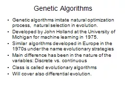
2. GA Quick OverviewDeveloped: USA in the 1970’sEarly names: J. Holland, K. DeJong, D. GoldbergTypically applied to: discrete optimizationAttributed features:not too fastgood heuristic for combinatorial problemsSpecial Features:Traditionally emphasizes combining information from good parents (crossover)many variants, e.g., reproduction models, operators

3. Genetic algorithmsHolland’s original GA is now known as the simple genetic algorithm (SGA)Other GAs use different:RepresentationsMutationsCrossoversSelection mechanisms

4. SGA technical summary tableauRepresentationBinary stringsRecombinationN-point or uniformMutationBitwise bit-flipping with fixed probabilityParent selectionFitness-ProportionateSurvivor selectionAll children replace parentsSpecialityEmphasis on crossover

5. Genotype space = {0,1}LPhenotype spaceEncoding (representation)Decoding(inverse representation)0111010010100010011001001010010001Representation

6. SGA reproduction cycleSelect parents for the mating pool (size of mating pool = population size)Shuffle the mating poolFor each consecutive pair apply crossover with probability pc , otherwise copy parentsFor each offspring apply mutation (bit-flip with probability pm independently for each bit)Replace the whole population with the resulting offspring

7. SGA operators: 1-point crossoverChoose a random point on the two parentsSplit parents at this crossover pointCreate children by exchanging tailsPc typically in range (0.6, 0.9)

8. SGA operators: mutationAlter each gene independently with a probability pm pm is called the mutation rateTypically between 1/pop_size and 1/ chromosome_length

9. Main idea: better individuals get higher chanceChances proportional to fitnessImplementation: roulette wheel techniqueAssign to each individual a part of the roulette wheel Spin the wheel n times to select n individualsSGA operators: Selectionfitness(A) = 3fitness(B) = 1fitness(C) = 2AC1/6 = 17%3/6 = 50%B2/6 = 33%

10. An example after Goldberg ‘89 (1)Simple problem: max x2 over {0,1,…,31}GA approach:Representation: binary code, e.g. 01101  13Population size: 41-point xover, bitwise mutation Roulette wheel selectionRandom initialisationWe show one generational cycle done by hand

11. x2 example: selection

12. X2 example: crossover

13. X2 example: mutation

14. The simple GAHas been subject of many (early) studiesstill often used as benchmark for novel GAsShows many shortcomings, e.g.Representation is too restrictiveMutation & crossovers only applicable for bit-string & integer representationsSelection mechanism sensitive for converging populations with close fitness valuesGenerational population model (step 5 in SGA repr. cycle) can be improved with explicit survivor selection

15. Alternative Crossover OperatorsPerformance with 1 Point Crossover depends on the order that variables occur in the representationmore likely to keep together genes that are near each otherCan never keep together genes from opposite ends of stringThis is known as Positional BiasCan be exploited if we know about the structure of our problem, but this is not usually the case

16. n-point crossoverChoose n random crossover pointsSplit along those pointsGlue parts, alternating between parentsGeneralisation of 1 point (still some positional bias)

17. Uniform crossoverAssign 'heads' to one parent, 'tails' to the otherFlip a coin for each gene of the first childMake an inverse copy of the gene for the second childInheritance is independent of position

18. Crossover OR mutation?Decade long debate: which one is better / necessary / main-background Answer (at least, rather wide agreement):it depends on the problem, butin general, it is good to have bothboth have another rolemutation-only-EA is possible, xover-only-EA would not work

19. Exploration: Discovering promising areas in the search space, i.e. gaining information on the problemExploitation: Optimising within a promising area, i.e. using informationThere is co-operation AND competition between them Crossover is explorative, it makes a big jump to an area somewhere “in between” two (parent) areas Mutation is exploitative, it creates random small diversions, thereby staying near (in the area of ) the parentCrossover OR mutation? (cont’d)

20. Only crossover can combine information from two parentsOnly mutation can introduce new information (alleles)Crossover does not change the allele frequencies of the population (thought experiment: 50% 0’s on first bit in the population, ?% after performing n crossovers)To hit the optimum you often need a ‘lucky’ mutationCrossover OR mutation? (cont’d)

21. Other representationsGray coding of integers (still binary chromosomes)Gray coding is a mapping that means that small changes in the genotype cause small changes in the phenotype (unlike binary coding). “Smoother” genotype-phenotype mapping makes life easier for the GANowadays it is generally accepted that it is better to encode numerical variables directly asIntegersFloating point variables

22. Integer representationsSome problems naturally have integer variables, e.g. image processing parameters Others take categorical values from a fixed set e.g. {blue, green, yellow, pink}N-point / uniform crossover operators workExtend bit-flipping mutation to make“creep” i.e. more likely to move to similar valueRandom choice (esp. categorical variables)For ordinal problems, it is hard to know correct range for creep, so often use two mutation operators in tandem

23. Real valued problemsMany problems occur as real valued problems, e.g. continuous parameter optimisation f :  n  Illustration: Ackley’s function (often used in EC)

24. Mapping real values on bit stringsz  [x,y]   represented by {a1,…,aL}  {0,1}L[x,y]  {0,1}L must be invertible (one phenotype per genotype): {0,1}L  [x,y] defines the representation Only 2L values out of infinite are representedL determines possible maximum precision of solutionHigh precision  long chromosomes (slow evolution)

25. Floating point mutations 1General scheme of floating point mutations Uniform mutation: Analogous to bit-flipping (binary) or random resetting (integers)

26. Floating point mutations 2Non-uniform mutations:Many methods proposed,such as time-varying range of change etc.Most schemes are probabilistic but usually only make a small change to valueMost common method is to add random deviate to each variable separately, taken from N(0, ) Gaussian distribution and then curtail to rangeStandard deviation  controls amount of change (2/3 of deviations will lie in range (-  to + )

27. Crossover operators for real valued CRsDiscrete:each allele value in offspring z comes from one of its parents (x,y) with equal probability: zi = xi or yi Could use n-point or uniformIntermediateexploits idea of creating children “between” parents (hence a.k.a. arithmetic recombination)zi =  xi + (1 - ) yi where  : 0    1. The parameter  can be:constant: uniform arithmetical crossovervariable (e.g. depend on the age of the population) picked at random every time

28. Single arithmetic crossoverParents: x1,…,xn  and y1,…,ynPick a single gene (k) at random, child1 is:reverse for other child. e.g. with  = 0.5

29. Simple arithmetic crossoverParents: x1,…,xn  and y1,…,ynPick random gene (k) after this point mix valueschild1 is:reverse for other child. e.g. with  = 0.5

30. Most commonly usedParents: x1,…,xn  and y1,…,ynchild1 is:reverse for other child. e.g. with  = 0.5Whole arithmetic crossover

31. Permutation RepresentationsOrdering/sequencing problems form a special typeTask is (or can be solved by) arranging some objects in a certain order Example: sort algorithm: important thing is which elements occur before others (order)Example: Travelling Salesman Problem (TSP) : important thing is which elements occur next to each other (adjacency)These problems are generally expressed as a permutation:if there are n variables then the representation is as a list of n integers, each of which occurs exactly onceInitially skip!!

32. Permutation representation: TSP exampleProblem:Given n citiesFind a complete tour with minimal lengthEncoding:Label the cities 1, 2, … , nOne complete tour is one permutation (e.g. for n =4 [1,2,3,4], [3,4,2,1] are OK)Search space is BIG: for 30 cities there are 30!  1032 possible tours

33. Mutation operators for permutationsNormal mutation operators lead to inadmissible solutionse.g. bit-wise mutation : let gene i have value jchanging to some other value k would mean that k occurred twice and j no longer occurred Therefore must change at least two valuesMutation parameter now reflects the probability that some operator is applied once to the whole string, rather than individually in each position

34. Insert Mutation for permutationsPick two allele values at randomMove the second to follow the first, shifting the rest along to accommodateNote that this preserves most of the order and the adjacency information

35. Swap mutation for permutationsPick two alleles at random and swap their positionsPreserves most of adjacency information (4 links broken), disrupts order more

36. Inversion mutation for permutationsPick two alleles at random and then invert the substring between them.Preserves most adjacency information (only breaks two links) but disruptive of order information

37. Scramble mutation for permutationsPick a subset of genes at randomRandomly rearrange the alleles in those positions(note subset does not have to be contiguous)

38. “Normal” crossover operators will often lead to inadmissible solutionsMany specialised operators have been devised which focus on combining order or adjacency information from the two parentsCrossover operators for permutations1 2 3 4 55 4 3 2 11 2 3 2 15 4 3 4 5

39. Order 1 crossoverIdea is to preserve relative order that elements occurInformal procedure:1. Choose an arbitrary part from the first parent2. Copy this part to the first child3. Copy the numbers that are not in the first part, to the first child:starting right from cut point of the copied part, using the order of the second parent and wrapping around at the end4. Analogous for the second child, with parent roles reversed

40. Order 1 crossover exampleCopy randomly selected set from first parentCopy rest from second parent in order 1,9,3,8,2

41. Informal procedure for parents P1 and P2:Choose random segment and copy it from P1 Starting from the first crossover point look for elements in that segment of P2 that have not been copiedFor each of these i look in the offspring to see what element j has been copied in its place from P1Place i into the position occupied j in P2, since we know that we will not be putting j there (as is already in offspring)If the place occupied by j in P2 has already been filled in the offspring k, put i in the position occupied by k in P2Having dealt with the elements from the crossover segment, the rest of the offspring can be filled from P2. Second child is created analogouslyPartially Mapped Crossover (PMX)

42. PMX exampleStep 1Step 2Step 3

43. Cycle crossoverBasic idea: Each allele comes from one parent together with its position.Informal procedure:1. Make a cycle of alleles from P1 in the following way. (a) Start with the first allele of P1. (b) Look at the allele at the same position in P2.(c) Go to the position with the same allele in P1. (d) Add this allele to the cycle.(e) Repeat step b through d until you arrive at the first allele of P1.2. Put the alleles of the cycle in the first child on the positions they have in the first parent.3. Take next cycle from second parent

44. Cycle crossover exampleStep 1: identify cyclesStep 2: copy alternate cycles into offspring

45. Edge RecombinationWorks by constructing a table listing which edges are present in the two parents, if an edge is common to both, mark with a +e.g. [1 2 3 4 5 6 7 8 9] and [9 3 7 8 2 6 5 1 4]

46. Edge Recombination 2Informal procedure once edge table is constructed1. Pick an initial element at random and put it in the offspring2. Set the variable current element = entry3. Remove all references to current element from the table4. Examine list for current element:If there is a common edge, pick that to be next elementOtherwise pick the entry in the list which itself has the shortest listTies are split at random5. In the case of reaching an empty list:Examine the other end of the offspring is for extensionOtherwise a new element is chosen at random

47. Edge Recombination example

48. Multiparent recombinationRecall that we are not constricted by the practicalities of natureNoting that mutation uses 1 parent, and “traditional” crossover 2, the extension to a>2 is natural to examineBeen around since 1960s, still rare but studies indicate useful Three main types:Based on allele frequencies, e.g., p-sexual voting generalising uniform crossoverBased on segmentation and recombination of the parents, e.g., diagonal crossover generalising n-point crossoverBased on numerical operations on real-valued alleles, e.g., center of mass crossover, generalising arithmetic recombination operators

49. Population ModelsSGA uses a Generational model:each individual survives for exactly one generationthe entire set of parents is replaced by the offspringAt the other end of the scale are Steady-State models: one offspring is generated per generation, one member of population replaced,Generation Gap the proportion of the population replaced1.0 for GGA, 1/pop_size for SSGAResume Discussion here!

50. Fitness Based CompetitionSelection can occur in two places:Selection from current generation to take part in mating (parent selection) Selection from parents + offspring to go into next generation (survivor selection)Selection operators work on whole individuali.e. they are representation-independentDistinction between selectionoperators: define selection probabilities algorithms: define how probabilities are implemented

51. Implementation example: SGAExpected number of copies of an individual i E( ni ) =  • f(i)/ f ( = pop.size, f(i) = fitness of i, f avg. fitness in pop.)Roulette wheel algorithm:Given a probability distribution, spin a 1-armed wheel n times to make n selectionsNo guarantees on actual value of ni Baker’s SUS algorithm:n evenly spaced arms on wheel and spin onceGuarantees floor(E( ni ) )  ni  ceil(E( ni ) )

52. Problems includeOne highly fit member can rapidly take over if rest of population is much less fit: Premature ConvergenceAt end of runs when fitness is similar, lose selection pressure Highly susceptible to function transpositionScaling can fix last two problemsWindowing: f’(i) = f(i) -  t where  is worst fitness in this (last n) generationsSigma Scaling: f’(i) = max( f(i) – ( f  - c • f ), 0.0)where c is a constant, usually 2.0Fitness-Proportionate Selection

53. Function transposition for FPS

54. Rank – Based SelectionAttempt to remove problems of FPS by basing selection probabilities on relative rather than absolute fitnessRank population according to fitness and then base selection probabilities on rank where fittest has rank  and worst rank 1This imposes a sorting overhead on the algorithm, but this is usually negligible compared to the fitness evaluation timeInitially skip!!

55. Linear RankingParameterised by factor s: 1.0 < s  2.0measures advantage of best individualin GGA this is the number of children allotted to it Simple 3 member example

56. Exponential RankingLinear Ranking is limited to selection pressureExponential Ranking can allocate more than 2 copies to fittest individualNormalise constant factor c according to population size

57. Tournament SelectionAll methods above rely on global population statisticsCould be a bottleneck esp. on parallel machinesRelies on presence of external fitness function which might not exist: e.g. evolving game players Informal Procedure:Pick k members at random then select the best of theseRepeat to select more individualsResume!

58. Tournament Selection 2Probability of selecting i will depend on:Rank of iSize of sample k higher k increases selection pressureWhether contestants are picked with replacementPicking without replacement increases selection pressureWhether fittest contestant always wins (deterministic) or this happens with probability pFor k = 2, time for fittest individual to take over population is the same as linear ranking with s = 2 • p

59. Survivor SelectionMethods developed for parent selection can be reusedSurvivor selection can be divided into two approaches:Age-Based Selectione.g. SGAIn SSGA can implement as “delete-random” (not recommended) or as first-in-first-out (a.k.a. delete-oldest) Fitness-Based SelectionUsing one of the methods above or

60. Two Special CasesElitismWidely used in both population models (GGA, SSGA)Always keep at least one copy of the fittest solution so farGENITOR: a.k.a. “delete-worst”From Whitley’s original Steady-State algorithm (he also used linear ranking for parent selection)Rapid takeover : use with large populations or “no duplicates” policy