5.0 Discrete-time Fourier Transform - PowerPoint Presentation

Slide1

5.0 Discrete-time Fourier Transform

5.1 Discrete-time Fourier Transform Representation for discrete-time signals

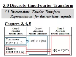
Chapters 3, 4, 5

Chap 3 PeriodicFourier SeriesChap 4 Aperiodic Fourier Transform Chap 5 Aperiodic Fourier Transform

Continuous

Discrete

 Slide2

Fourier

Transform (p.3 of 4.0)

T FS

  0 

 periodic in  discrete in

 aperiodic in   

continuous in

T

 Slide3

Discrete-time Fourier Transform

0

periodic in

 aperiodic in

discrete and periodic in

continuous and periodic in

 Slide4

Harmonically Related Exponentials for Periodic

Signals

(p.11 of 3.0)

[n][n]

(N)

(N)

integer multiples of

ω

0‧Discrete in frequency domainSlide5
Slide6
Slide7
Slide8

From Periodic to Aperiodic

Considering x[n], x[n]=0 for n > N

2 or n < -N1

ConstructSlide9

Fourier series for

From Periodic to AperiodicConsidering x[n], x[n]=0 for n >

N2 or n < -N1

Defining envelope of Slide10

As

From Periodic to AperiodicConsidering x[n], x[n]=0 for n >

N2 or n < -N1

signal, time domain, Inverse Discrete-time Fourier Transform

spectrum, frequency domain Discrete-time Fourier Transform

Similar format to all Fourier analysis representations previously discussedSlide11

Considering

x(t), x(t)=0 for | t | > T1 (p.10 of 4.0)

as

spectrum, frequency domainFourier Transform

signal, time domain Inverse Fourier Transform

Fourier Transform pair, different expressions

very similar format to Fourier Series for periodic signalsSlide12

Note:

X(ejω) is continuous and periodic with period 2Integration over 2 onlyFrequency domain spectrum is continuous and periodic, while time domain signal is discrete-time and aperiodicFrequencies around ω=0 or 2

are low-frequencies, while those around ω=  are high-frequencies, etc.From Periodic to AperiodicConsidering x[

n], x[n]=0 for n > N2 or n < -N1

See Fig. 5.3, p.362 of text For Examples see Fig. 5.5, 5.6, p.364, 365 of textSlide13
Slide14
Slide15
Slide16
Slide17

From Periodic to Aperiodic

Convergence Issuesgiven x[n]No convergence issue since the integration is over an finite intervalNo Gibbs phenomenon

See Fig. 5.7, p.368 of textSlide18
Slide19
Slide20
Slide21

Rectangular/SincSlide22

Fourier Transform for Periodic Signals –

Unified Framework (p.14 of 4.0)Given x(t)

(easy in one way)Slide23

Unified

Framework (p.15 of 4.0)

T FS

 Slide24

Fourier Transform for Periodic Signals –

Unified Framework (p.16 of 4.0)If

FSlide25

From Periodic to Aperiodic

For Periodic Signals – Unified FrameworkGiven x[n]

See Fig. 5.8, p.369 of textSlide26
Slide27

From Periodic to Aperiodic

For Periodic Signals – Unified FrameworkIf

See Fig. 5.9, p.370 of textSlide28
Slide29

5.2 Properties of Discrete-time Fourier

Transform

Periodicity

LinearitySlide30

Time/Frequency Shift

ConjugationSlide31
Slide32

Differencing/Accumulation

Time ReversalSlide33

Differentiation

(p.28 of 4.0)

Enhancing higher frequenciesDe-emphasizing lower frequencies

Deleting DC term ( =0 for ω=0)  

 Slide34

Integration

(p.29 of 4.0)

Accumulation

Enhancing lower frequencies (accumulation effect)De-emphasizing higher frequencies (smoothing effect)Undefined for ω=0

dc term

 Slide35

Differencing/Accumulation

Enhancing higher frequencies

De-emphasizing lower

freqDeleting DC termDifferencing/AccumulationSlide36

Time Reversal

(p.32 of 3.0)

unique representation

for orthogonal basisTime ReversalSlide37

Time Expansion

If n/k is an integer, k: positive integer

See Fig. 5.14, p.378 of text

See Fig. 5.13, p.377 of textSlide38
Slide39
Slide40

Time Expansion

 Slide41

Time Expansion

 Slide42

Differentiation in Frequency

Parseval’s RelationSlide43

Convolution Property

Multiplication Property

frequency response or transfer function

periodic convolutionSlide44

Input/Output

Relationship

 Time DomainFrequency Domain

00 

matrix vectors

eigen

value

eigen

vector

(

P.51

of

4.0

)Slide45

Convolution Property

(

p.53 of 4.0)Slide46

System Characterization

Tables of Properties and Pairs

See Table 5.1, 5.2, p.391, 392 of textSlide47
Slide48
Slide49

Vector Space Interpretation

basis signal sets

{x[n], aperiodic defined on -∞ < n < ∞}=V is a vector space

repeats itself for very 2

Slide50

Generalized

Parseval’s Relation

inner-product can be evaluated in either domain

Vector Space Interpretation{X(ejω), with period 2π defined on -∞ < ω < ∞}=

V : a vector spaceSlide51

Orthogonal Bases

Vector Space InterpretationSlide52

Orthogonal Bases

Similar to the case of continuous-time Fourier transform. Orthogonal bases but not normalized, while makes sense with operational definition.

Vector Space InterpretationSlide53

Signal Representation in Two Domains

Time Domain Frequency Domain

, k: integer,

 Slide54

Summary and Duality

(p.1 of 5.0)

Chap 3 PeriodicFourier SeriesChap 4 Aperiodic Fourier Transform

Chap 5 Aperiodic Fourier Transform Continuous <C>

 <A>

<D>

Discrete <B>

 Slide55

5.3 Summary and Duality

<A> Fourier Transform for Continuous-time Aperiodic Signals

(Synthesis) (4.8)

(Analysis) (4.9)-x(t) : continuous-time aperiodic in time(∆t→0) (T→∞)

-X(jω) : continuous in aperiodic infrequency(ω0→0) frequency(W→∞)

Duality<A> : Slide56

00

Case <A> (

p.40 of 4.0)

 0

 Slide57

<B> Fourier Series for Discrete-time Periodic Signals

(Synthesis) (3.94)

(Analysis) (3.95)-x[

n] : discrete-time periodic in time(∆t = 1) (T = N)-ak : discrete in periodic infrequency(ω0 = 2 / N) frequency(W = 2

)

Duality<B> : Slide58

Case <B> Duality

 Slide59

<C> Fourier Series for Continuous-time Periodic Signals

(Synthesis) (3.38)

(Analysis) (3.39)-x(

t) : continuous-time periodic in time(∆t → 0) (T = T)-ak : discrete in aperiodic infrequency(ω0 = 2 / T) frequency(W

→ ∞)Slide60

Case <C> <D> Duality

<C>

<D> 

 0

0

0 1 2 3

For <C>

For <D>

Duality Slide61

<D> Discrete-time Fourier Transform for Discrete-time

Aperiodic Signals

(Synthesis) (5.8)(Analysis) (5.9)-x

[n] : discrete-time aperiodic in time(∆t = 1) (T→∞)-X(ejω) : continuous in periodic infrequency(ω0→0) frequency(W = 2)Slide62

<D> Discrete-time Fourier Transform for Discrete-time

Aperiodic SignalsDuality<C> / <D>

For <C>For <D>Duality

taking

z

(t) as a periodic signal in time with period 2,

substituting into (3.38), ω0 = 1which is of exactly the same form of (5.9) except for a sign change, (3.39) indicates how the coefficients ak are obtained, which is of exactly the same form of (5.8) except for a sign change, etc.

See Table 5.3, p.396 of textSlide63
Slide64

More Duality

Discrete in one domain with

∆ between two values→ periodic in the other domain with period Continuous in one domain (∆ → 0)→ aperiodic in the other domain

  Slide65

[n]

[n]

(N)

(N)

integer multiples of

ω0

‧

Discrete in frequency domain

Harmonically Related Exponentials for Periodic Signals (p.11 of 3.0)Slide66

Extra Properties Derived from Duality

examples for Duality <B>

duality

dualitySlide67

Unified Framework

Fourier Transform : case <A>

(4.8)(4.9)Slide68

Unified Framework

Discrete frequency components for signals periodic in time domain: case <C>

you get (3.38)

(applied on (4.8))Case <C> is a special case of Case <A>Slide69

Fourier Transform for Periodic Signals –

Unified Framework (p.16 of 4.0)If

FSlide70

Unified Framework

Discrete time values with spectra periodic in frequency domain: case <D>

(4.9) becomesNote : ω in rad/sec for continuous-time but in rad for

discrete-time(5.9)

Case <D> is a special case of Case <A>Slide71

Time

Expansion (p.41 of 5.0)

 Slide72

Unified Framework

Both discrete/periodic in time/frequency domain: case <B> -- case <C> plus case <D>

periodic and discrete, summation over a period of N

(4.8) becomes (4.9) becomes

(3.94) (3.95) Slide73

Unified Framework

Cases <B> <C> <D> are special cases of case <A>Dualities <B>, <C>/<D> are special case of Duality <A>Vector Space Interpretation----similarly unifiedSlide74

Examples

Example 5.6, p.371 of textSlide75

Examples

Example 4.8, p.299 of text

(

P.73 of 4.0)Slide76

Examples

Example 5.11, p.383 of text

time shift propertySlide77

Examples

Example 5.14, p.387 of textSlide78
Slide79
Slide80

Examples

Example 5.17, p.395 of textSlide81

Examples

Example 3.5, p.193 of text

(a)

(b)(c)

(P. 60 of 3.0)Slide82

Problem 5.36(c)

, p.411 of textSlide83

Problem

5.36(c), p.413 of textSlide84

Problem 5.46

, p.415 of textSlide85

Problem 5.56

, p.422 of textSlide86

Problem 3.70

, p.281 of text

2-dimensional signals

(P. 67 of 3.0)Slide87

Problem 3.70

, p.281 of text

2-dimensional signals

(P. 66 of 3.0)Slide88

An Example across Cases <A><B><C><D>Slide89

Time/Frequency Scaling

(p.31 of 4.0)

See Fig. 4.11, p.296 of text

inverse relationship between signal “width” in time/frequency domainsexample: digital transmission (required bandwidth) α (bit rate)Slide90

Time/Frequency Scaling

(

p.32

of 4.0)Slide91

Parseval’s

Relation (p.30

of 4.0)total energy: energy per unit time integrated over the time

total energy: energy per unit frequency integrated over the frequency 

 Slide92

Single Frequency

(

p.34

of 4.0)Slide93

Single FrequencySlide94

Another ExampleSlide95

Cases <C><D>Slide96

Cases <B>