Spectral Lines - PowerPoint Presentation

Slide1

Spectral Lines

Robert MinchinSlide2

Spectral Lines

What is a Spectral Line?

Types of Spectral Line

Molecular Transitions

Linewidths

Reference FramesSlide3

When a Coconut falls…

Bang!

h

Energy released =

mghSlide4

When an electron falls…

J = 1/2

F=1

F=0

e

-

𝛾

Energy carried away by photon: E =

hν

Flash!

Transition energy ∝ photon frequency

⇒ Spectral Lines!Slide5

n

= 2

Energy levels

J = 1/2

F=1

F=0

J = 1/2

F=1

F=0

J = 3/2

F=2

F=1

n

= 1

Fine Structure:

spin-orbit coupling

Atomic levels:

electron shells

Hyperfine Structure:

coupling of nuclear and

electron magnetic dipolesSlide6

H

I

n

= 2

Energy levels

J = 1/2

F=1

F=0

J = 1/2

F=1

F=0

J = 3/2

F=2

F=1

n

= 1

Ly

α

Ultra-violet

Microwave

Note: Ly

α

is actually a doublet due to the fine structure splitting Slide7

Types of Spectral Line

Spontaneous Emission

Absorption

Stimulated EmissionSlide8

Spontaneous Emission

The electron decays to a lower energy level without any particular trigger

Stochastic process

Likelihood given by Einstein A coefficient:

A

ulIn general, these are smaller in the radio than in the optical:

H I (21-cm): Aul = 2.7 × 10-15 s

-1Ly α (121.6 nm): Aul = 5 × 108

s-1Slide9

The H I

hyperfine transition

CENSOREDSlide10

The H I

hyperfine transition

S

pin parallel → spin anti-parallel

Predicted in 1944

Detected in 1951Very low probability: A

ul = 2.7 × 10-15 s-1 But generally get NHI

≥ 1020 cm-2 in galaxiesGet ~105 transitions per second per cm

2Population maintained by collisions

This is the column we look down

with our telescopesSlide11

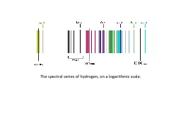
Recombination Lines

Lyman

α

:

n

= 2 → n = 1 – 122 nmBalmer α:

n = 3 → n = 2 – 656 nmPaschen α:

n = 4 → n = 3 – 1870 nmBrackett α: n = 5 →

n = 4 – 4050 nmPfund α: n = 6 →

n = 5 – 7460 nmHumphreys α

: n = 7 → n = 6 – 12400 nmSlide12

Recombination Lines

Lyman

α

:

n

= 2 → n = 1 – 122 nmLyman β:

n = 3 → n = 1 – 103 nmLyman γ: n = 4 →

n = 1 – 97.3 nmLyman δ: n = 5 → n = 1 – 95.0 nm

Lyman ε: n = 6 → n = 1 – 93.8 nmLyman limit:

n = ∞ → n = 1 – 91.2 nmSlide13

Recombination Lines

Bigger jumps = more energy = shorter

λ

Bigger jumps are also less likely to occur

Higher levels = less energy = longer

λHigher levels less likely to be populatedHigher lines are denoted

Hnα, Hnβ, etc., where

n is the final energy levelSlide14

Recombination Lines

Frequencies can be calculated using:

ν

= 3.28805 × 10

15

Hz (1/nl2 – 1/n

u2) This gives frequencies in the radio (ν < 1 THz) for (1/nl2

– 1/nu2) < 3 × 10-4This is met for Hn

α when n > 19, for Hnβ when

n > 23, etc.Known as Radio Recombination Lines (RRLs

)Also get RRLs from He and CSlide15

n

=10

n

=9

n

=8

n

=7

n

=6

Coconut Rolling

n

=5

n

=4

n

=3

n

=2

n

=1

BANG!

Bang!

Bang

BUMP

Bump

Bump

Bump

Bump

BumpSlide16

n

=172

n

=171

n

=170

n

=169

n

=168

Coconut Rolling

n

=167

n

=166

n

=165

n

=164

Bang

n

=163

Bang

Bang

Bang

Bang

Bang

Bang

Bang

Bang

In the radio, the steps in energy are much more evenSlide17

n

=172

n

=171

n

=170

n

=169

n

=168

Coconut Rolling

n

=167

n

=166

n

=165

n

=164

n

=163

In the radio, the steps in energy are much more even

1304 MHz

1327 MHz

1350 MHz

1375 MHz

1399 MHz

1425 MHz

1451 MHz

1477 MHz

1505 MHzSlide18

Absorption

The electron is kicked up to a higher energy level by absorbing a photon

Likelihood given by Einstein B coefficient and the radiation density:

B

lu

Uν(T)

Blu is proportional to Aul/νul3

– Absorption becomes more important at lower frequenciesAbsorption is often more likely than spontaneous emission in the radioSlide19

Stimulated Emission

Sometimes called ‘negative absorption’

The electron is stimulated into giving up its energy by a passing photon

Likelihood given by Einstein B coefficient and the radiation density:

B

ul U

ν(T) Bul is also proportional to Aul/

νul3 – Stimulated emission becomes more important at lower frequenciesSlide20

Absorption vs Stimulated Emission

e

-

Photons that are at the right frequency to be

absorbed are also at the right frequency to

stimulate emissionSlide21

Absorption vs Stimulated Emission

B

ul

= (

g

l/g

u) Blugl and g

u are the statistical weights of the lower and upper energy levelsThe populations – in thermal equilibrium - are given by thermodynamics:Nu/

Nl = (gu/gl

) e-(h

ν/kTex)T

ex is the excitation temperature – not always the same thing as the physical temperatureSlide22

Absorption vs Stimulated Emission

If a background source has a

radiation temperature

T

bg

, then if T

bg > Tex we getNu/

Nl < (gu/gl)

e-(hν/kTbg)

This means absorption can take place – if the photons actually hit the absorberAlso need the absorbing medium to be ‘optically thick’

The photons from the background source are likely to hit something, rather than going straight through Slide23

Optically Thick

(If you can stay out of the gutter!)

Optical ThicknessSlide24

Optical Thickness

Optically Thin

(Poor odds of hitting anything)Slide25

Optical Thickness

What fraction of a background source is absorbed depends on the optical depth,

τ

This depends on the column density of the absorbing medium

Can therefore use the fractional absorption to measure the column densitySlide26

Funky Formaldehyde

Collisions between formaldehyde (H

2

CO) and water (H

2

O) molecules can anti-pump formaldehyde into its lowest energy stateThis causes a ‘negative inversion’, which can have a very low excitation temperatureWhen it falls below the temperature of the CMB, formaldehyde can be seen in absorption anywhere in the universe!Slide27

Funky Formaldeyde

H

2

CO absorption against the CMB from

Zeiger

& Darling (2010)

CMB is 4.6 K at this zUpper line is 2 cm (GBT) at 1.5 – 2 KLower line is 6cm (AO) at ~ 1KSlide28

Absorption vs Stimulated Emission

Like the anti-pumping in Formaldehyde, can have pumping that

causes N

u

/

Nl

> (gu/gl)As Nu

/Nl = (gu/g

l) e-(hν/kT

ex), this means Tex

< 0 This is a maser (or a laser in the optical)Microwave (Light) Amplification by Stimulated Emission of RadiationAstrophysically

important masers include OH (hydroxyl), water (H20), and methanol (CH3OH)Slide29

Conjugate Lines

To within the noise, the lines sum to zero

What’s going on?Slide30

Conjugate Lines

2

Π

3

/2

, J=3/2

-

F=2

F=1

+

F=2

F=1

Λ

- doubling

This is due to the interaction between

the molecule’s rotation and electron spin-orbit motion. It occurs in diatomic radicals like OH and gives ‘main lines’ and ‘satellite lines’

The ground state of OH:

Main lines

1665 MHz

1667 MHz

1720 MHz

1612 MHz

Satellite linesSlide31

Conjugate Lines

The hyperfine levels of the OH ground state are populated by electrons falling (‘cascading’) from higher levels

These higher levels are excited by – and compete for – FIR photons

The two possible transitions to the ground state are:

2

Π3/2

, J=5/2 → 2Π3/2, J=3/2 (intra-ladder) 2Π1/2

, J=1/2 → 2Π3/2, J=3/2 (cross-ladder)Slide32

Conjugate Lines

Only certain transitions are allowed, therefore:

A cascade through

2

Π

3/2, J=5/2 will give an over-population in the F=2 hyperfine levelsA cascade through 2

Π1/2, J=1/2 will give an over-population in the F=1 hyperfine levelsOver-population in F=2 gives masing at 1720 MHz and absorption at 1612 MHzOver-population in F=1 gives

masing at 1612 MHz and absorption at 1720 MHz Slide33

Conjugate Lines

Which route dominates is determined by when the transitions become optically thick

Below a column-density of N

OH

/ΔV ~ 10

14 cm-2, we don’t get conjugate lines

For NOH/ΔV ~ 1014 – 1015 cm-2, get 1720 MHz in emission, 1612 MHz in absorption

Above NOH/ΔV ~ 1015 cm-2, get 1612 MHz in emission, 1720 in absorptionSlide34

Molecular Transitions

Electronic

Vibrational

RotationalSlide35

Molecular Transitions

Electronic transitions are analogous to those in the hydrogen atom.

Vibrational

transitions are due to electronic forces between pairs of nucleiSlide36

Vibrational

Transitions

Rocking

Wagging

Scissoring

Asymmetrical

Stretching

Twisting

Symmetrical

Stretching

Vibrations of CH

2

, by Tiago

Bercerra Paolini, source: Wikimedia CommonsSlide37

Molecular Transitions

Electronic transitions are analogous to those in the hydrogen atom.

Vibrational

transitions are due to electronic forces between pairs of nuclei

Rotational transitions due to different modes in which the molecules can rotateSlide38

Rotational Transitions

SO

2

and H

2

0 animations from The Astrochymist, www.astrochymist.orgSlide39

Molecular Transitions

Approximate ratio of energies is:

1 : (m

e

/m

p)1/2 : m

e/mp(electronic : vibrational : rotational)

Only vibrational and rotational lines are seen with radio telescopes Many molecular lines are seen at sub-mm and mm wavelengths

‘Lab Astro’ needed to find accurate frequenciesSlide40

Find frequencies via NRAO’s

catalogue at http://

www.splatalogue.orgSlide41

Linewidths

Natural

Random Motions

Ordered MotionsSlide42

Natural Linewidth

Broadening due to Heisenberg’s uncertainty principle

P

roportional to the transition probability:

A

ulProduces a ‘Lorentzian

’ profile – more strongly peaked than a Gaussian, with higher wingsThis is important in the optical, but is normally negligible in the radio, as Aul is usually smallSlide43

Random Internal Motions

Intrinsic to the source region, not the line

Maxwell-Boltzmann distribution

Thermal motions: σ

v,thermal

2 = kTk

/mMicro-turbulence: σv,turb2 = vturb2/2

Add in quadrature: σv2 = kTk

/m + vturb2/2 Define ‘Doppler temperature’, TD, such that:

σv2

= kTD/m = kTk/m + v

turb2/2 This is what we can actually determineSlide44

Random Internal Motions

σ

v

= (kT

D

/m)

1/2

FWHM = 2 (2 ln(2))

1/2 σv

Slide45

Ordered Internal Motions

Inflow/ContractionSlide46

Ordered Internal Motions

Outflow/ExpansionSlide47

Ordered Internal Motions

Rotating DiscSlide48

Ordered Internal Motions

Rotating DiscSlide49

Inflow

Simulated spectrum of inflowing gas in the envelope of a

protostar

From

Masunaga

& Inutsuka (2000)1: Initial condition

6: Just after first core forms12: Early stage of main accretion phase13: Late stage of main accretion phaseSlide50

Expanding Shell

Continuum-subtracted HI spectrum of an expanding shell in M101

From

Chakraborti

& Ray (2011) / THINGS

Interpret double peaks as approaching and receding hemispheres of the shellSlide51

Rotating DiscSlide52

External Motions

If the source is in motion relative to us (or we are in motion relative to it) then its observed frequency will be

D

oppler shifted

This does not change the width of the source (although it may appear to at relativistic recession velocities)

The motion of the source is defined w.r.t. a reference frameSlide53

Reference Frames

Topocentric

Geocentric

Barycentric

(Heliocentric)Local Standard of Rest

Other FramesInertial frames w.r.t. the universeSlide54

Topocentric

The velocity frame of the observer – you!

Other velocity frames must be transformed to

topocentric

to make accurate observations

Varies with 1 day (Earth’s rotation) and 1 year (Earth’s orbit) periods w.r.t. astronomical sourcesLocal RFI is stationary in this frameSlide55

A

Topocentric

ImageSlide56

Geocentric

Reference frame of the centre of the Earth

Differs from

topocentric

by up to ~0.5 km s

-1, depending on time, pointing direction and latitudeVaries with 1 year period w.r.t. astronomical sources Slide57

A Geocentric Image

Rotating Earth by

Wikiscient

, from NASA images. Source: Wikimedia CommonsSlide58

Barycentric (Heliocentric)

‘Heliocentric’ refers to the centre of the Sun, ‘

b

arycentric

’ to the Solar System

barycentre (centre of mass)Barycentric is normally used in modern astronomy, heliocentric is historical

Differ from geocentric by up to ~30 km s-1, depending on time and pointing directionUsed for most extra-galactic spectral line workSlide59

A

Barycentric

ImageSlide60

Local Standard of Rest (LSR)

Inertial transform from

barycentric

– depends only on position on the sky

Based on average motion of local stars – removes the peculiar velocity of the Sun

(Kinematic LSR, Dynamic LSR is in circular motion around the Galactic centre)Differs from barycentric

by up to ~20 km s-1Used for most Galactic spectral-line workSlide61

An LSR ImageSlide62

Other Frames

Galactocentric

– motion of the Galactic centre

Local Group – motion of the Local Group

CMB Dipole – rest-frame of the CMB

Source – rest frame of the sourceThis can be useful in looking at source structure

Particularly useful for sources at relativistic velocitiesAll of these are inertial on the sorts of timescales we are worried aboutSlide63

Defining Velocity

It sounds simple – how fast a thing is moving away from us (or towards us)

Redshift

is defined as being the shift in wavelength divided by the rest wavelength:

z

= (λ

obs – λrest)/λrest = Δλ/λ

rest From this, get the optical definition of velocity: vopt

= czThis is not a physical definition!

vopt > c for

z > 1Slide64

Defining Velocity

An alternative ‘radio velocity’ definition is:

v

radio

=

c(νrest –

νobs)/νrest =

cΔν/νrestOptical velocity can be also be written in terms of frequency using:

vopt = cΔν/

νobsThis allows observing frequency to be calculated as:

νobs = νrest

(1 + νopt/c)-1 = νrest (1 – νradio

/c)Slide65

Relativistic Velocity

True (relativistic) velocity is given by:

v

rel

=

c (ν

rest2 – νobs2)/(ν

rest2 + νobs2)Frequency can be found

relativistically using:νobs = ν

rest(1 - (|v|/c)

2)1/2/(1 + v⋅s/c)

(v is velocity vector, s is the unit vector towards source)As we normally only know v⋅s

, not v, this is usually simplified (with v = v⋅

s) to:νobs = νrest

(1 - (v/c)2)1/2/(1 + v/c)Slide66

So we know the frequency, right?

Not quite – we need to shift from whatever frame the velocity was in to

topocentric

First find frequency in desired frame:

ν

frAlso need the

topocentric velocity of the frame at the time of the observation: vfrNow find topocentric frequency using:

νtopo = νfr(1 – (|

vfr|/c)2)1/2/(1 + v

fr⋅s/c

)Slide67

Velocity vs Frequency

A 1 MHz shift in frequency corresponds to a change in velocity in km s

-1

equal

†

to the rest wavelength in mm

δv/(km s-1

) = λ/mm × δν/MHz

†in the radio velocity conventionSlide68

You should now know:

How spectral lines form

How to find their rest frequencies

How they get their line widths/profiles

How to calculate observing frequencies

So – what can you actually do with them?Slide69

Lots to Learn from Lines

Chemical properties - abundances & composition

Physical properties – temperature & density

Ordered motions of sources

Rotation of galaxies

Infall regions & outflow regionsVelocities of sourcesTrace spiral arms of the Milky Way

Distances to external galaxies – the 3D universe!Slide70