
amp Coincident Site Lattice CSL Theory Texture Microstructure amp Anisotropy AD Rollett Last revised 20 th Mar 16 2 Objectives The objectives of this lecture are Develop an understanding of grain boundary engineering ID: 529035
Download Presentation The PPT/PDF document "1 Grain Boundary Engineering" is the property of its rightful owner. Permission is granted to download and print the materials on this web site for personal, non-commercial use only, and to display it on your personal computer provided you do not modify the materials and that you retain all copyright notices contained in the materials. By downloading content from our website, you accept the terms of this agreement.


Slide1
1
Grain Boundary Engineering& Coincident Site Lattice (CSL) Theory
Texture, Microstructure & AnisotropyA.D. Rollett
Last revised: 20th Mar. ‘16Slide2
2
ObjectivesThe objectives of this lecture are:Develop an understanding of grain boundary engineeringExplain the theory of Coincident Site Lattices (CSLs) and how it applies to grain boundariesShow how microstructures are analyzed for CSL contentSlide3
3
References on Grain BoundariesInterfaces in Crystalline Materials, Sutton & Balluffi, Oxford U.P., 1998. Very complete compendium on interfaces.
Interfaces in Materials, J. Howe, Wiley, 1999. Useful general text at the upper undergraduate/graduate level.Crystal Defects and Crystalline Interfaces,
W. Bollmann, (1970). New York, Springer Verlag.
Grain Boundary Migration in Metals, G. Gottstein and L.
Shvindlerman
, CRC Press, 1999. The most complete review on grain boundary migration and mobility.
Materials Interfaces: Atomic-Level Structure & Properties
, D. Wolf & S. Yip, Chapman & Hall, 1992.
Bollmann
, W. (
1982),
Crystal lattices, interfaces, matrices
. Published by the author,
Geneva.
Grimmer, H
.,
Disorientations and coincidence rotations for cubic lattices.
Acta
Crystall
.
A30
(1974) 685–688.
Grimmer, H
.,
Bollmann
, W
.,
Warrington, D. H
.,
Coincidence- site lattices and complete pattern-shift lattices in cubic crystals.
Acta
Cryst
.
A30
(1974) 197 – 207
.
Bonnet, R.,
et al
. (1981). Determination of near-Coincident Cells Hexagonal Crystals - Related DSC Lattices.
Acta
Crystall
.
A37
184-189.
Ikuhara
, Y. and P.
Pirouz
(1996). Orientation relationship in large mismatched
bicrystals
and coincidence of reciprocal lattice points (CRLP). In:
Intergranular and
Interphase
Boundaries in Materials, Pt 1
.
207
121-124.Slide4
References on GBE
The main point of these references is that the annealing twins only increase in density during primary recrystallization and that they are created as the recrystallization fronts advance through the material. There is also the paper by Lin et al. that shows that the one exception to this statement is that new twin-related grains are occasionally created at triple lines during grain growth. All this in fcc metals (only).“Evolution of the Annealing Twin Density during δ-Supersolvus Grain Growth in the Nickel-Based Superalloy Inconel™ 718”, Yuan Jin, Marc Bernacki, Andrea Agnoli, Brian Lin, Gregory S. Rohrer, Anthony D. Rollett and Nathalie Bozzolo, Metals, 6, 5 (2016); doi:10.3390/met6010005.
“Annealing Twins in Nickel Nucleate at Triple Lines During Grain Growth”, B. Lin, Y. Jin, C.M. Hefferan, S.F. Li, J. Lind, R.M. Suter, M. Bernacki
, N. Bozzolo, A.D. Rollett, G.S. Rohrer, Acta Materialia, 99, 63-68 (2015); doi:10.1016/j.actamat.2015.07.041.“Thermo-Mechanical Factors Influencing Annealing Twin Development In Nickel During Recrystallization”, Y. Jin, B. Lin, A.D. Rollett, G.S. Rohrer, M.
Bernacki, N. Bozzolo, Journal of Materials Science 50
5191-5203 (2015).
"Annealing twin development during recrystallization and grain growth in pure Nickel", Y. Jin, B. Lin, M.
Bernacki
, G.S. Rohrer, A.D. Rollett, N.
Bozzolo
,
Materials Science and Engineering: A
,
597 295–303 (2014). Miller, H. M., C.-S. Kim, J. Gruber, V. Randle and G. S. Rohrer (2007). "Orientation Distribution of sigma-3 Grain Boundary Planes in Ni Before and After Grain Boundary Engineering." Materials Science Forum 558-559: 641-647.Rohrer, G. S., V. Randle, C. S. Kim and Y. Hu (2006). "Changes in the five-parameter grain boundary character distribution in alpha-brass brought about by iterative thermomechanical processing." Acta materialia 54(17): 4489-4502.
4Slide5
5
OutlineSlides from Integran with examples of Grain Boundary Engineered materialsCSL theoryBrandon’s criterion for classification of grain boundaries by CSL typeTechnical information on comparative properties of GBE and non-GBE materialsSlide6
Reading
Pages 3-25 of Sutton & BalluffiPages 307-346 of Howe.6Slide7
7
Grain Boundary EngineeringGrain Boundary Engineering (GBE) is the practice of obtaining microstructures with a high fraction of boundaries with desirable properties.In general, desirable properties are associated with boundaries that have simple, low energy structures.Such low energy structures are, in turn, associated with CSL boundaries.GBE generally consists of repeated cycles of deformation and annealing, chosen so as to generate large fractions of “special boundaries” and avoid development of strong recrystallization textures.
GBE is largely confined at present to fcc metallic systems such as stainless steel, nickel alloys,
Pb, Cu.Note that detailed information on exactly which CSL boundaries have useful properties is lacking, as is information on how the typical processing routes actually produce high fractions of CSL boundaries.Slide8
8
Metallurgical Nano-Technology Nanocrystalline materials
are those in which the average crystal size is reduced 1000-fold from the micron-range in conventional materials to the nanometer size range (3-100nm). This can be cost -effectively achieved by proprietary electrodeposition techniques (NanoPlate™).
Grain boundary engineering (GBE™) is the methodology by which the local grain boundary structure is characterized and material processing variables adjusted to create an optimized grain boundary microstructure for improved material performance.
Courtesy of:Slide9
9
GBE Technology
Patent-Protected Thermo-Mechanical Metallurgical Process
Applied during component forming/fabrication processes.
Can also be applied as a surface treatment (0.1 to 1mm) to finished or semi-finished structures.
Increases Population of ‘Special’ Grain Boundaries
Reduces Average Grain Size
Enhances Microstructural Uniformity
Fully Randomizes Crystallographic Texture
GBE Surface Treatment
Alloy 625
Special GB’s (
red
;
yellow
)
General GB’s
(
black
)
Grain boundary engineering
(GBE™) is the methodology by which the local grain boundary structure is characterized and material processing variables adjusted to create an optimized grain boundary microstructure for improved material performance.
Base Material
Integran’s GBE technology has also been applied to mitigate stress corrosion cracking susceptibility of Ni-base alloys, extend the service-life of lead-acid battery grids, and improve the fatigue and creep performance of aerospace superalloys.Slide10
10
0.02 in.
0.02”
0.02”
Conventional
Nuclear Steam Generator Tubing
Cross sections of sample gauge lengths following interrupted environmental CERT tests.
Test Conditions: 60h; 10% NaOH; 600F; +0.100 mV vs. OCP; Ni Ref. Electrode; 5X10
-7
in/sec.
Alloy 690 nuclear steam generator tubing can be further optimized for SCC-resistance by GBE mill processing technology. Alloy 690 is replacing 600 in many nuclear power plants because of its enhanced resistance to SCC.
See also:
Alexandreanu
, B., B.
Capell
, et al. (2001). "Combined effect of special grain boundaries and grain boundary carbides on IGSCC of Ni-16Cr-9Fe-xC alloys."
Materials Science and Engineering
A
300
(1-2):
94.Slide11
11
Lead-Acid Batteries
Conventional lead-acid battery grid (Pb-1wt%Sb) following 4 years of service.
The cycle - life of lead-acid batteries (e.g., automotive) is compromised by intergranular degradation processes (corrosion, cracking).
Conventional
(fsp<15%) after 2 weeks of cycling.
GBE
(fsp=55%) after 4 weeks of cycling.
Integran’s innovative GBE
®
grid processing technology is designed to extend the service life of conventional SLI and industrial batteries (US Patent No. 6,342,110 B1).
Palumbo, G
.
et
al
. (1998). "Applications for grain boundary engineered materials."
Journal of Minerals, Metallurgy and Materials (JOM)
50
40-43.Slide12
12
Corrosion of Aluminum 2124Results from experiment involving intergranular corrosion of aluminum alloy 2124. Low angle boundaries are measurably more resistant than high angle boundaries. Some evidence for resistance of 3 and
7 boundaries (possibly also 3).
Research (unpublished) by Lisa Chan, CMU.See also (e.g.): Tan, L., Allen, T.R. and Busby, J.T., 2013. Grain boundary engineering for structure materials of nuclear reactors. Journal of Nuclear Materials, 441(1), pp.661-666.Slide13
13
Corrosion in NiGertsman et al., Acta Mater., 49 (9): 1589-1598 (2001).
Several
3 boundaries with larger deviations from ideal misorientation cracked.
Alloy 600 (Ni-base alloy)Slide14
14
S3 Boundaries14
Lin et al., Acta Metall. Mater.
, 41 (2): 553-562 (1993).
Cracked
3 boundaries were found to deviate more than 5°from the trace of the {111} plane.
Ni
3
AlSlide15
15
Fatigue
0
2
0
0
0
0
0
4
0
0
0
0
0
6
0
0
0
0
0
8
0
0
0
0
0
1
0
0
0
0
0
0
1
2
0
0
0
0
0
A
l
l
o
y
6
2
5
/
6
0
k
s
i
A
l
l
o
y
7
3
8
/
4
0
k
s
i
V
5
7
/
4
0
k
s
i
R
o
o
m
T
e
m
p
e
r
a
t
u
r
e
F
a
t
i
g
u
e
P
e
r
f
o
r
m
a
n
c
e
o
f
S
e
l
e
c
t
e
d
N
i
c
k
e
l
B
a
s
e
d
A
l
l
o
y
s
C
o
n
v
e
n
t
i
o
n
a
l
G
B
E
Cycles to Failure
M
a
t
e
r
i
a
l
/
S
t
r
e
s
sSlide16
16
Creep
Alloy V57
Alloy 625
Conventional
GBE
Thaveeprungsriporn
, V. and G. S. Was (1997). "The role of coincidence-site-lattice boundaries in creep of Ni-16Cr-9Fe at 360 degrees C."
Metallurgical And Materials Transactions
A
28
(10):
2101;
Alexandreanu
, B
.
et al. (2003). "The effect of grain boundary character distribution on the high temperature deformation behavior of Ni-16Cr-9Fe alloys."
Acta
materialia
51
3831.Slide17
17
Special Grain BoundariesThere are some boundaries that have special properties, e.g. low energy.In most known cases (but not all!), these boundaries are also special with respect to their crystallography.When a finite fraction of lattice sites coincide between the two lattices, then one can define a coincident site lattice (CSL).A boundary that contains a high density of lattice points in a CSL is expected to have low energy because of good atomic fit.
Note that the boundary plane matters, in addition to the misorientation; this means, in effect, that only pure tilt or pure twist boundaries are likely to have a high density of CSL lattice points.Relevant website:
http://www.tf.uni-kiel.de/matwis/amat/def_en/kap_7/illustr/a7_1_1.html (a page from a general set of pages on defects in crystals: http://www.tf.uni-kiel.de/matwis/amat/def_en/index.html ).Slide18
18
Grain Boundary propertiesFigure taken from Gottstein & Shvindlerman, based on Goux, C. (1974). “Structure des joints de grains: consideration cristallographiques
et methodes de calcul des structures.” Canadian Metallurgical Quarterly
13: 9-31.]For example,
fcc <110> tilt boundaries show pronounced minima in energyHowever, some caution needed because the <100> series do
not
show these minima.
S
3
60°<111>
S
11
50°<110>Slide19
19
Kronberg & WilsonKronberg & Wilson in 1949 considered coincidence patterns for atoms in the boundary planes (as opposed to the coincidence of lattice sites). Their atomic coincidence patterns for 22° and 38° rotations on the 111 plane correspond to the S
13b and S7 CSL boundary types. Note the significance of coincidence in the plane of the boundary.
Friedel also explored CSL-like structures in a study of twins.Kronberg, M. L. and F. H. Wilson (1949), “Secondary recrystallization in copper”,
Trans. Met. Soc. AIME, 185, 501-
514.
Friedel
, G. (1926).
Lecons
de
Cristallographie
(2nd ed.). Blanchard, Paris. Slide20
20
Sigma=5, 36.9° <100>[Sutton & Balluffi]Slide21
21
CSL = geometrical conceptThe CSL is a geometrical construction based on the geometry of the lattice.Lattices cannot actually overlap!If a (fixed) fraction of lattice sites are coincident, then the expectation is that the boundary structure will be more regular than a general boundary.Atomic positions are not
accounted for in CSLs.It is possible to compute the density of coincident sites in the plane of the boundary - this goes beyond The basic CSL concept, which has to do only with the lattice misorientation.Slide22
22
CSL constructionThe rotation of the second lattice is limited to those values that bring a (lattice) point into coincidence with a different point in the first lattice.The geometry is such that the rotated point (in the rotated lattice 2) and the superimposed point (in the fixed lattice 1) are related by a mirror plane in the unrotated state.Slide23
23
Rotation to CoincidenceRed and Green lattices coincide
Points to be brought into coincidenceSlide24
24
rotating to the S5 relationshipSlide25
25
rotating to the
S
5 relationshipSlide26
26
rotating to the
S
5 relationshipSlide27
27
rotating to the
S
5 relationshipSlide28
28
rotating to the
S
5 relationshipSlide29
29
rotating to the
S
5 relationshipSlide30
30
rotating to the
S
5 relationshipSlide31
31
rotating to the
S
5 relationshipSlide32
32
rotating to the
S
5 relationshipSlide33
33
S5 relationshipRed and Green lattices coincide after rotation of 2 tan-1 (1/3) = 36.9° Slide34
34
Rotation to achieve coincidence
Rotate lattice 1 until a lattice point in lattice 1 coincides with a lattice point in lattice 2.
Clear that a higher density of points observed for low index axis.
[Bollmann, W. (1970). Crystal Defects and Crystalline Interfaces. New York, Springer Verlag.]Slide35
35
CSL rotation angleThe angle of rotation can be determined from the lattice geometry. The discrete nature of the lattice means that the angle is always determined as follows. q
= 2 tan-1 (y
/x),
where
(
x
,
y
)
are the coordinates of the superimposed point (in 1);
x
is measured parallel to the mirror plane.
y
xSlide36
36
CSL <-> RodriguesYou can immediately relate the angle to a Rodrigues vector because the tangent of the semi-angle of rotation must be rational (a fraction, y/x); thus the magnitude of the corresponding Rodrigues vector must also be rational!Example: for the
S5 relationship, x=3 and
y=1; thus q = 2 tan-1
(y/
x
) = 2 tan
-1
(1/3)
= 36.9°
and the rotation axis is
[1,0,0]
, so the complete Rodrigues vector =
[1/3, 0, 0]. Slide37
37
The Sigma value (S)Define a quantity, S', as the ratio between the area enclosed by a unit cell of the coincidence sites, and the standard unit cell. For the cubic case that whenever an even number is obtained for S', there is a coincidence lattice site in the center of the cell which then means that the true area ratio,
S, is half of the apparent quantity. Therefore S
is always odd in the cubic system.Slide38
38
Generating functionStart with a square lattice. Assign the coordinates of the coincident points as (n,m)*: the new unit cell for the coincidence site lattice is square, each side is √(
m2+n2
) long. Thus the area of the cell is m2+n
2. Correct for m
2
+n
2
even: there is another lattice point in the center of the cell thereby dividing the area by two.
*
n
and
m
are identical to x and y
discussed in previous slidesSlide39
39
Range of m,nRestrict the range of m and n such that
m<n.If n=m
then all points coincide, and m>n does not produce any new lattices.Example of
5: m
=1,
n
=3,
area
=(3
2
+1
2
) = 10; two lattice points per cell, therefore volume ratio = 1:5; rotation angle =2 tan-1
1/3 = 36.9°
.
m
nSlide40
40
Generating function, contd.Generating function: we call the calculation of the area a generating function.
Sigma denotes the ratio of the volume of coincidence site lattice to the regular latticeSlide41
41
Generating function: RodriguesA rational Rodrigues vector can be generated by the following expression, where {m,n,h,k,l} are all integers, m<n.
r
= m/n [h,k,l]The rotation angle is then:
tan
q
/2
=
m/n
√
(
h
2+k2+l
2
)Slide42
42
Sigma ValuesA further useful relationship for CSLs is that for sigma. Consider the rotation in the (100) plane:
tan{q/2} =
m/narea of CSL cell = m
2+n2
=
n
2
(1 + (m/n)
2
) = n
2
(1 + tan2{
q
/2
})
Extending this to the general case, we can write:
S
=
n
2
(1 + tan
2
{
q
/2
}) =
n
2
(
1 +
{
m/n
√(
h
2
+k
2
+l
2
)}
2
) =
n
2
+ m
2
(
h
2
+k2
+l
2
)
Note that although using these formulas and inserting low order integers generates most of the low order
CSLs
,
one must go to values of n~5 to obtain
a complete list.
[
Ranganathan
, S. (1966). “On the geometry of coincidence-site lattices.”
Acta
Crystallographica
21
197-
199; see also the
Morawiec
book, pp 142-149 for discussion of cubic and lower symmetry cases]Slide43
Quaternions
Recall that all CSL relationships can be thought of as twin relationships, which means that (in a centrosymmetric lattice) they can be constructed as 180° rotations about some axis. Rotations of 180° have a very simple representation as a quaternion (by contrast to Rodrigues vectors) because cos(q/2)=cos(90°)=0 and sin(
90°)=1. Therefore for a rotation axis of [x,y,z
] the unit quaternion (for 180°) = {x,y,z,0}.Take the S5 as an example. The rotation axis is [310], therefore the quaternion representation is
1/√10{3,1,0,0}.
Check that this is indeed the expected value by applying symmetry to the ∆g and indeed one finds that this is equivalent to
{1/3,0,0}
as a Rodrigues vector or
38.9°[100]
.
One can further check that a vector of type [310] is mapped onto its negative by using the quaternion to transform/rotate it. If we choose [-1,3,0] as being orthogonal to the [310] axis, we can use the standard formula. PTO…
43Slide44
Quaternions, contd.
Note that q0 = 0 in these cases (of 180° rotations) and q2=1, so that simplifies the formula considerably:s = -v + 2(v•q) q
= -v + 2(
v•[310]) [310]Pick [-1,3,0] as an example: = -
v + 2
([-1,3,0
]
•
[
3,1,0
]) [
3,1,0]
= -v + 2([-3+3+0]) [3,1,0]
=
[+1,-3,0
]
Note that any value of the z coefficient will
also
satisfy the relationship.
Note that any combination of
b=-3a
in
[
a,b,c
]
(i.e. that has integer coordinates to be a point in the lattice, and is perpendicular to the axis) will also work. This helps to make the point that there is an infinite set of points that coincide, each of which satisfies the required relationship. That infinite set of coincident points is the Coincident Site
Lattice
.
44Slide45
45
Table of CSL values in axis/angle, Euler angles, Rodrigues vectors
and quaternions
Note: in order to compare a measured misorientation with one of these values, it is necessary to compute the values to high precision (because most are fractions based on integers).
Note: integer fractions are quoted for most of the Rodrigues vectors. The entries in decimals also correspond to integer values and will be updated at a later time.Slide46
46
CSL + boundary planeGood atomic fit at an interface is expected for boundaries that intersect a high density of (coincident site) lattice points.How to determine these planes for a given CSL type?The coincident lattice is aligned such that one of its axes is parallel to the misorientation axis. Therefore there are two obvious choices of boundary plane to maximize the density of CSL lattice points:
(a) a pure twist boundary with a normal // misorientation axis is one example, e.g. (100) for any <100>-based CSL;
(b) a symmetric tilt boundary that lies perpendicular to the axis and that bisects the rotation should also contain a high density of points. Example: for S5, 36.9° about <001>,
x=3, y=1, and so the (310) plane corresponds to the S
5
symmetric tilt boundary
plane,
i.e
. (
n,m,0
).Slide47
47
CSL boundaries and RF spaceThe coordinates of nearly all the low-sigma CSLs are distributed along low index directions, i.e. <100>, <110> and <111>. Thus nearly all the CSL boundary types are located on the edges of the space and are therefore easily located. There are some CSLs on the 210, 331 and 221 directions, which are shown in the interior of the space.Slide48
48
RF pyramid and CSL locations
l
=100
l
=110
l
=111
R
1
+R
2
+R
3
=1
(
√
2-1,0)
(
√
2-1,
√
2-1)Slide49
Plan View:
Projection on R
3= 0
49<110>,
<111>
<100>
<111>
line
lies over the
<110>
line
33cSlide50
50
Fractions of CSL Boundaries in a Randomly Oriented MicrostructureIt is interesting is to ask what fraction of boundaries correspond to each sigma value in a randomly oriented polycrystal?
The method to calculate such (area) fractions is exactly the same as for volume fractions in an Orientation Distribution.
The Brandon Criterion establishes the “capture radius” for each sigma value (which decreases with increasing sigma value).All points (in a discretized MD) are assigned to a given CSL type if they fall within the capture radius.Slide51
51
CSL % for Random Texture
Garbacz
et al.
, Scr. Mater.,
23
(8): 1369-1374 (1989).
Gertsman
et al.
,
Acta
Metall. Mater.,
42
(6): 1785-1804 (1994).
Morawiec
et. al.
,
Acta
Metall. Mater.,
41
(10): 2825-2832 (1993).
Pan
et al.
, Scr. Metall. Mater.,
30
(8): 1055-1060 (1994).
Generate MD from a random texture; analyze for fraction near each CSL type (method to be discussed later).Slide52
Grain Boundaries from High Energy Diffraction Microscopy
Measurements made at the Advanced Photon Source: see Hefferan et al. (2009). CMC 14
209-219.Pure Nickel: 42 layers, 4 micron spacing, 0.16 mm3
Pure Ni sample, 42 layers
3,496 grains; ~ 23,598 GBsSlide53
Statistics extraction from large data sets
Neighbor misorientation angle distribution
Hefferan
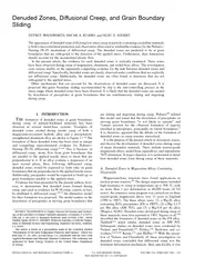
et al. (2009). CMC 14 209-219.Slide54
S27
aStatistics extraction from large data sets
Neighbor misorientation angle distribution
S27b
S7
S3
Conclusion:
The misorientations of grain boundaries in these nickel samples are concentrated on a small number of CSL types, i.e. sigma = 3,7,9,11,27
Hefferan
et al
. (2009). CMC
14
209-219.Slide55
55
Brandon CriterionDavid Brandon [ 1966: "The structure of high-angle grain boundaries”, Acta metallurgica
14: 1479-1484] originated a criterion for proximity to a CSL structure.
vm = v
0S
-1/2
where the proportionality constant, v
0
, is generally taken to be 15°, based on the low-to-high angle transition.
Larger sigma values imply larger unit cells in the boundary, fewer coincident points, larger dislocation densities for the same deviation from the exact CSL misorientation. Thus one has to closer to the exact CSL position in order for a given boundary to be counted as belonging to that CSL type.
Closeness to a misorientation type is defined by the angle associated with the rotation between the misorientation in question,
∆g
, and the CSL misorientation,
∆
g
CSL
.
cos
(
m
) = {trace(∆g ∆
g
T
CSL
)-1}/2Slide56
56
Impact of the Brandon CriterionSlide57
57
Brandon Criterion, contd.Thus, if: qm
< v0S
m-1/2 < 15°m-1/2
then we accept the
boundary as belonging
to the CSL of type
S=
m
.
The justification is
based on the existence
of a dislocation structure for vicinal interfaces to CSL structures, just as for low angle boundaries [see fig. 2.33 from Sutton & Balluffi]. Typical cutoff at
S=
29.Slide58
58
How near to a CSL?A reasonable way to measure distance from a special boundary type and an arbitrarily specified boundary is to calculate a minimum rotation angle (“orientation distance”) in exactly the same way as for the disorientation. In terms of Rodrigues vectors, we write the following for the composition of two rotations, r1r2, which represents
r1 followed by r
2:Slide59
59
Composition of Rodrigues vectorsTo use this, we simply assign the components of a CSL boundary type to one of the Rodrigues vectors (strictly speaking, the inverse rotation, although the negative rotation is always equivalent to the positive one.
As always, one must use the crystal symmetry operators in order to find the smallest available angle.
Unless both the CSL value
and
the misorientation have been placed in the fundamental zone, then one will obtain the wrong result
.Slide60
60
Angle from CSLOne can then extract the angle, q, from the length of the resultant vector (Chapter 3), where r is the Rodrigues vector description of the boundary in question and |r| is the rotation angle associated with the vector:
q0
= |r • r
000/0°| = |r
•
r
S1
|,
r
S1
=(0,0,0)q1 = |r
•
r
111/60°
| = |
r
•
r
S3
|,
r
S3
=(1/3,1/3,1/3)
q
3
= |
r
•
r
111/38.21°
| ,
r
S7
=(0.2,0.2,0.2)Slide61
61
Deviation from a CSLThe deviation of a given misorientation from an exact misorientation type, such as a CSL type, is found by forming the product of the misorientation to be tested, and the inverse of the reference type.Given a ∆g = (OBg
B)(OA
gA)-1, and a reference type, ∆g
CSL, then form the product
∆g’ = ∆g (∆g
CSL
)
-1
.
As stated before, it is necessary to apply
all
the relevant (crystal) symmetry operators (including the switching symmetry) to the ∆g in order to ensure that the variant that is closest to the reference type is included in the comparison. This means that the result must be chosen that produces the minimum angle
and
that places the misorientation axis in the fundamental zone.
Given the product “mis-misorientation”, one usually only considers the magnitude (rotation angle) extracted from it.
All these operations can be performed with matrices, Rodrigues vectors, or (unit) quaternions. Most serious software uses quaternions.Slide62
62
Algorithm for Disorientation: 1To find the disorientation*, as just an angle, associated with a grain boundary but not identifying which symmetry operator was required for each crystal:Make a list of all crystal symmetry operators;
Loop over switching symmetry (2 passes), which computes both ∆gAB
and ∆gBA ;Loop over
OA (24 different operators, for cubic crystal symmetry);
Calculate
∆g
=
g
B
(
O
A
gA)-1 or (OAgA) gB-1 and extract the angle (e.g. as arc-cosine of [trace(
∆g
)-1]/2),
depending on the first loop;
If (misorientation) angle is lower than the previous result then retain the result (as the current candidate for the disorientation);
End of loops: the misorientation that satisfied the tests is the disorientation because it possesses the minimum rotation angle. The misorientation axis can be placed in a
single standard
stereographic triangle by making all the indices positive that are associated with the minimum angle, and re-ordering so as to make
h≤k≤l
, for example.
*Disorientation:= combination of minimum angle and axis located in the fundamental zoneSlide63
63
Algorithm for Disorientation: 2To find the disorientation* associated with a grain boundary and identify which symmetry operator on each crystal provided the disorientation (useful for analyzing 5-parameter grain boundary character:List all relevant symmetry operators;Compute both ∆gAB
and ∆gBA (for switching symmetry);
first loop over switching symmetry (2 passes);Second loop over OA ;Third loop over OB to calculate ∆g
= (OB
g
B
)(
g
A
O
A
)
-1 or (OAgA)(gBOB)-1
, depending on the first loop;
If (misorientation) rotation axis associated with
∆g
lies within the fundamental zone (e.g. 100-110-111 SST for cubic), then proceed to the next test (treat the first such finding as a special case, i.e. retain the result and do
not
apply the next test);
If
(misorientation) angle is lower than the previous result then retain the result (as the current candidate for the disorientation);
End
of loops: the misorientation that satisfied the tests is the disorientation because it lies within the fundamental zone and possesses the minimum rotation angle
.
For any subsequent calculations, e.g. of boundary normal, ensure that you use the same symmetry operator in each grain as was found to yield the disorientation.
*Disorientation:= combination of minimum angle and axis located in the fundamental zoneSlide64
64
Example: Effect of GBCD on Pb Electrodes in Lead-Acid BatteriesPalumbo et al. [Palumbo, G., E. M. Lehockey, and P. Lin (1998). “Applications for grain boundary engineered materials.” JOM
50(2): 40-43.
] have shown that the crystallographic nature of grain boundaries in Pb have a strong effect on the resistance of Pb electrodes (in the form of lattice-work grids) to failure via
intergranular corrosion and creep-cracking. More specifically, Pb
that has been processed to have a high fraction of special boundaries, i.e. coincidence site lattice boundaries with low sigma numbers, exhibit significantly longer lifetimes. Slide65
65
Pb electrodes, contd.The figure (next slide) illustrates the difference in performance for Pb-Ca-Sn-Ag lead-acid positive battery grids following 40 charge-discharge cycles. The image on the left is the as-cast material with 7% special boundaries (3 S 29); the image on the right is the grain boundary engineered material with 67.6% special boundaries. The small amount of Ca added to Pb is a hardening agent (from the eutectic at 0.07% Ca).Slide66
66Slide67
67
Example: creep resistance in Inconel 600: Ni-16Cr-9FeCreep resistance of Ni-alloys is strongly enhanced by maximizing the fraction of special boundaries.Solution annealed (SA) vs. CSL-enhanced (CSLE): note higher frequencies of low- boundaries.
Was, G. S., V. Thaveepringsriporn, et al. (1998). “Grain boundary misorientation effects on creep and cracking in Ni-based alloys.” JOM
50(2): 44-49.Slide68
68
Creep ResistanceConstant load creep curves show dramatic improvement in creep resistance from samples with normal boundaries, and [grain boundary engineered] GBE samples with a high fraction of CSL boundaries.
Grain Boundary Engineered
Standard MaterialSlide69
69
Creep RatesCreep resistance thought to be enhanced by resistance of CSL boundaries to recovery of extrinsic dislocations. Lack of recovery in CSLs means higher back stresses opposing creep stress, therefore lower strain rate.Slide70
70
Thaveepringsriporn, V. and Was, G. S. (1997). “The role of CSL boundaries in creep of Ni-16Cr
-9Fe at 360°C.” Metall. Trans.
28A: 2101.Mechanism
Dislocations (extrinsic grain boundary dislocations) accumulate in CSL boundaries giving rise to back stresses that oppose creep.Slide71
71
Creep of Ni: modelThe creep rate as a function of grain size and boundary type was modeled (after Sangal & Tangri) assuming that dislocation annihilation is much slower in CSL boundaries than in general boundaries.Slide72
72
V. Thaveepringsriporn and Was, G. S. (1997). “The role of CSL boundaries in creep of Ni-16Cr-9Fe
at 360°C.” Metall. Trans.
28A: 2101.Grain BoundaryCracking
Cracking at grain boundaries in corrosion testing post-creep shows strong sensitivity to boundary type: CSL boundaries are less prone to corrosion attack.Slide73
73
Grain Boundary PropertiesBased on these remarks on grain boundary structure, one might expect that CSL boundaries (especially in the pure twist or tilt boundary alignment) would have low energy because of good atomic fit.Some observations support this, e.g. deposition of small particles on a single crystal shows that low-sigma CSL boundaries are favored.“Grain boundary engineering” relies on simply maximizing the (area) fraction of CSL boundaries. This is typically made quantitative by adopting Brandon’s criterion and counting the fraction of boundaries that are associated with S
≤29.Observations of grain boundary character MgO
[Saylor & Rohrer] suggest otherwise: the low surface energy plane tends to dominate the grain boundary distribution, and is associated with low boundary energy in all crystalline materials.
It turns out that fcc metals are the exception because of their exceptionally low coherent twin boundary energy, which, in Ni & Cu (for example) is about 5% of the high angle GB energy. This promotes the formation of annealing twins, which in turn result in related CSL types being present such as
S
9,
S
27.Slide74
74
SummaryThe Coincident Site Lattice is a useful concept for identifying boundaries with low misfit (thus, low energy) in fcc metals.
Brandon’s criterion: Standard analysis of orientation distance leads to a criterion for how close a given grain boundary is to a particular CSL type. Brandon’s criterion
provides a numerical measure that is based on the concept of interfacial dislocations that accommodate small departures from an exact CSL relationship.Grain Boundary Engineering relies upon CSL analysis.Macroscopic Degrees of Freedom
: In general, five parameters needed to describe crystallographic grain boundary character. This is apparent in the combination of CSL misorientation relationship and twist or tilt boundary plane (to maximize CSL point density in the boundary plane).Caution
: the CSL theory applies to lattice sites, not atom positions.
Evidence
suggests
strongly
that
in all except
fcc
metals, the properties
are related to the two surfaces that make up the boundary, not the CSL structure. The existence of low energy boundaries for e.g.,
3 and
11 boundaries is “coincidence”.Slide75
Supplemental Slides
Information on CSL relationships in hcp metals, courtesy of Nathalie Bozzolo, CEMEF, France.75Slide76
CSL list for HCP
76Bozzolo et al. (2010). "Misorientations induced by deformation twinning in titanium." J. Appl. Crystallography
43 596-602Slide77
CSLs for HCP in RF space
77Note the two different conventions for alignment of the orthonormal coordinate system (used for calculations) with the crystallographic axes. Typically Channel (HKL) systems use the Y-convention whereas EDAX (TSL/OIM) systems use the X-convention.Certain CSL relationships correspond to deformation twins observed in Ti and
Zr.Bozzolo
et al. (2010). "Misorientations induced by deformation twinning in titanium." J. Appl. Crystallography 43 596-602