

Crossratios Twoview projective SFM Multiview geometry More projective SFM Planches httpwwwdiensfr poncegeomvislect4pptx httpwwwdiensfrponcegeomvislect4pdf ID: 555063
Download Presentation The PPT/PDF document "The end of projective cameras" is the property of its rightful owner. Permission is granted to download and print the materials on this web site for personal, non-commercial use only, and to display it on your personal computer provided you do not modify the materials and that you retain all copyright notices contained in the materials. By downloading content from our website, you accept the terms of this agreement.


Slide1
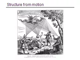
The end of projective cameras
Cross-ratios Two-view projective SFM Multi-view geometry More projective SFM
Planches
:
http://www.di.ens.fr/~
ponce/geomvis/lect4.pptx
http://www.di.ens.fr/~ponce/geomvis/lect4.pdfSlide2
Projective Spaces: (Semi-Formal) DefinitionSlide3
A Model of
P( R )3Slide4
Projective Subspaces and Projective CoordinatesSlide5
Affine and Projective SpacesSlide6
Affine and
ProjectiveCoordinatesSlide7
Affine and
ProjectiveCoordinatesSlide8
Cross-Ratios
Collinear points
Pencil of coplanar lines
Pencil of planes
{A,B;C,D}=
sin(
+
)sin(
+
)
sin(
+
+
)sin
Slide9
Cross-Ratios and Projective Coordinates
Along a line equipped with the basisIn a plane equipped with the basis
In 3-space equipped with the basis
*
*
*Slide10
Projective Transformations
Bijective linear map:
Projective transformation:
( = homography )
Projective transformations map projective subspaces onto
projective subspaces and preserve projective coordinates.
Projective transformations map lines onto lines and
preserve cross-ratios.Slide11
Perspective Projections induce projective transformations
between planes.Slide12
Projective Shape
Two point sets S and S’ in some projective space X are projectively equivalent
when there exists a projective
transformation y:
X
X
such that
S’ = y ( S ).
Projective structure from motion = projective shape recovery.
= recovery of the corresponding motion equivalence classes.Slide13
Epipolar
Geometry
Epipolar Plane
Epipoles
Epipolar Lines
BaselineSlide14
Geometric Scene
ReconstructionIdea: use (A,B,C,D,F) as a projective basis and reconstruct O’ and O’’, assuming that the epipolesare known.
A
B
C
D
F
G
H
I
J
K
E
O’
O’’Slide15
Geometric Scene
Reconstruction IIIdea: use (A,O”,O’,B,C)as a projective basis, assuming again that the
epipoles are known.Slide16
Epipolar Geometry
Epipolar Plane
Epipoles
Epipolar Lines
BaselineSlide17
Epipolar Constraint
Potential matches for p have to lie on the corresponding epipolar line l’.
Potential matches for
p’
have to lie on the corresponding
epipolar line
l
.Slide18
Epipolar Constraint: Calibrated Case
Essential Matrix
(
Longuet
-Higgins, 1981)Slide19
Properties of the Essential Matrix
E p’ is the epipolar line associated with p’. E p is the epipolar line associated with p. E e’=0 and E e=0. E is singular.
E has two equal non-zero singular values
(Huang and Faugeras, 1989).
T
TSlide20
Epipolar Constraint: Small Motions
To First-Order:
Pure translation:
Focus of ExpansionSlide21
Epipolar Constraint: Uncalibrated Case
Fundamental Matrix
(Faugeras and Luong, 1992)Slide22
Properties of the Fundamental Matrix
F p’ is the epipolar line associated with p’. F p is the epipolar line associated with p. F e’=0 and F e=0. F is singular.
T
TSlide23
The Eight-Point Algorithm (Longuet-Higgins, 1981)
|
F
|
=1.
Minimize:
under the constraint
2Slide24
Non-Linear Least-Squares Approach (Luong et al., 1993)
Minimize
with respect to the coefficients of F , using an
appropriate rank-2 parameterization.Slide25
The Normalized Eight-Point Algorithm (Hartley, 1995)
Center the image data at the origin, and scale it so themean squared distance between the origin and the data points is 2 pixels: q = T p , q’ =
T’ p’
.
Use the eight-point algorithm to compute F from the
points
q
and q’ . Enforce the rank-2 constraint.
Output T F T’
.Ti
ii
i
i
iSlide26
Data courtesy of R. Mohr and B. Boufama.Slide27
Without normalization
With normalization
Mean errors:
10.0pixel
9.1pixel
Mean errors:
1.0pixel
0.9pixel