Atmospheric tomography - PowerPoint Presentation

Slide1

Atmospheric

tomography of supergiant stars(starring μ Cep)

Alain Jorissen, Sophie Van Eck, Kateryna Kravchenko (Université Libre de Bruxelles)Andrea Chiavassa (Observatoire de la Côte d’Azur, Nice)Bertrand Plez (Université de Montpellier II)

Stellar End Products ESO, Garching, 2015

Based on observations carried out with the HERMES spectrograph

on the Mercator 1.2m telescope

Slide2

Region

I (innermost)Region III (outermost)X = log(τ500)Region II (middle)

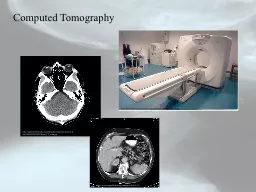
Tomography: I.1 techniqueAim is to probe velocity fields in stellar atmospheres Alvarez et al. (2000, A&A 362,655; 2001 A&A379, 288; 2001, A&A 379, 305) cross-correlate the observed

spectrum with numerical masks

probing

layers

of

increasing

depth

Construction

of the numerical masks :Computation of the depth function: τ500nm = C (λ; where τλ = 2/3)

Holes in mask IIprobing middle layer

Slide3

Instead

of imposing τλ = 2/3 for defining the mask holes, computation of « contribution function

 » expressing the depth of formation of spectral lines :

Tomography:

I

.2 technique (

improved

)

Albrow

&

Cottrell

(1996, MNRAS 278, 337): contribution function to the spectral-line flux depression:with Sl, I

c, μ, τ, κl, κ

c

taken from TURBOSPECTRUM (Alvarez & Plez 1998) using MARCS (1D) model atmospheres.

Slide4

Albrow

& Cottrell 1996Same spectral line, this workContribution function C(λ,τ) for the Fe I λ6546.245 line:

Sl, Ic, μ, τ, κl, κc taken from TURBOSPECTRUM (Alvarez & Plez 1998) using MARCS (1D) model atmosphere: Tomography

: I.3 technique (improved)

Slide5

For RSG:

Teff = 3490 K log g = -0.6 M = 12 M Solar composition Microturbulence 2 km/sSpectral resolution: Δλ = 0.01ÅContribution function C(λ,τ500 nm)

Computation of depth function: Cmax(λ) = τ500 of max C(λ,τ500) on all τ

Tomography

:

I

.4

technique

Relative flux

l

og

(τ500

)Cmax(λ)

Synthetic

spectrumWavelength (Å)

Crest line

Slide6

Computation of

depth function: Cmax(λ)= max C(λ,τ) (370 < λ (nm) < 910 ) for all τ

Atmosphere split in 8 vertical layersIn each layer, when Cmax(λ) is minimum (in τ500)Relative flux

Log(τ500)C

max

(λ

)

Synthetic

spectrum

Wavelength

(Å)

mask

hole

Tomography

:

I.5 technique (improved)…

Mask #8Mask #2

Mask #1

Slide7

Distribution of

linesin masks: -∞ -3 -2.5 -2 -1.5 -1 -0.5 0 +∞

InnermostOutermostAtmosphere temperature distributionTomography: I.6 techniqueMasks limits

MARCS synthetic spectrum

outer

inner

l

og

(τ

500

)

0.0

-0.5

-1.0-1.5-2.0-2.5

-3.0

-3.530002000 N

10000log(τ

500)10.9

10.710.51

0.410.210.21

0.1

Slide8

Tomography: II. Application to Miras

Cross-correlation of observed spectrum with mask function = CCF (Cross Correlation

Function)Follow the progression of a shock wave in the atmosphereSpatiallytemporally

time

outer

inner

a

tmospheric

depth

Alvarez et al. 2000, A&A 362,655

double-peak CCF

CCF

Slide9

Tomography: III. Interpretation

The Schwarzschild mechanismEvolution of Mira star CCFw

ith depthAlvarez et al. 2000, A&A 362,655Lagrangian description of the pulsating atmosphere

Slide10

Tomography: III. Interpretation

The Schwarzschild mechanismEvolution of Mira star CCFw

ith time atgiven depthAlvarez et al. 2000, A&A 362,655

time

outer

inner

a

tmospheric

depth

Lagrangian

description

of the pulsating atmosphere

Slide11

Tomography: IV. Application to sg

Same technique and masks, applied to supergiant starsNo cyclic behaviourSteep velocity gradients are observed on time scales of ~ 150 days

innerouterJosselin & Plez 2007, A&A 469, 671

Slide12

66 high-resolution (R = 86 000) spectra

of μ Cepobtained on the HERMES spectrograph (Raskin et al. 2011) on MERCATOR telescope (La Palma)Δt = 1505 d V. Application to μ Cep

Compute CCF (Radial Velocity)MARCS synthetic spectrum

outerinner

l

og

(τ

500

)

0.0

-0.5

-1.0

-1.5-2.0-2.5

-3.0-3.5μ Cep

Slide13

Innermost mask

Outermost mask0.0-0.5-1.0-1.5-2.0-2.5-3.0

-3.5log(τ500)The dance of the supergiant:Time lapse μ CepApril 2011 – Jan 2015

(see the attached file

tomo.mov

)

Slide14

Phase relation

between velocities and line depth (ratio)Gray, 2008, AJ 135, 1450BetelgeuseTypical time 400 d

μ CepObservation: 550 dLDR = Line Depth(VI)/Line Depth(FeI)Hysteresis (caused by convective cells

?)(km/s)

Slide15

t= 0 +90 +92 +133 +151 +161 +178 +190 d

Not quite the same behaviour as in Miras (above):In supergiants, the blue peak (ascending matter) never dominates→ in supergiants, the shock wave dies off rapidly, or is it a shock wave ?

Slide16

t= 0 +18 +65 +67 +80 +161 d

Another example, 450 d later

Slide17

inner

outer

Line doubling in deepest masksTomography: V. Velocity curve of μ Cep

matter falling down

m

atter

rising

CoM

velocity?

Max R

Min R

v = 0 km/s on the left scale !

Slide18

Line doubling in deepest masks

occurs during the

rising part of the light curveno data

Tomography: V. Velocity & light curves of μ Cep

Slide19

Hinkle,

Scharlach & Hall, 1984, ApJS 56, 1 Line doubling around max lightMax radius

recedingapproachingCO Δv = 3 linesTomography: VI. Situation in Mira variables (R Cas)

Slide20

Synthetic MARCS 1D

Synthetic CO5BOLD 3DObserved μ CepTomography

: VII. Comparison with 3D models

Slide21

Inner

Outer3D spectra: 4 OPTIM3D snapshots from CO5BOLD 3D models (Chiavassa

et al. 2011, A&A 535, A22)Teff = 3430 K M = 12 MR = 846 Rlog g = -0.35All

masks show consistent variations following radial-velocity curve

Tomography

:

VII.

Comparison

with

3D

models

Line doublingAAVSO photometry

Slide22

Observations

modelsOuterInner CCF depth

Inner masks sample weak linesOuter masks sample strong linesComparison with 3D CO5BOLD(4 snapshots): for outer masks especially:

3D CO5BOLD lines are deeper(factor ~1.5 to 2)

Depth

Slide23

Summary

COMPARISON WITH 3D MODELS:Some discrepancies for line depths, widths, & velocities (τ) currently being investigated by increasing numerical resolutionof models (Chiavassa et al.)A close collaboration

with 3D-modellers is needed to make the models reproduce all these data OBSERVED FEATURES: In the supergiant μ Cep, line doubling systematically occurs

on the rising part of the light curve; in the innermost

masks

;

is

never

seen in the outermost masks; with the red component stronger. Hysteresis between CCF/line depth and velocity

The evolution of line doubling is different in Miras and supergiants