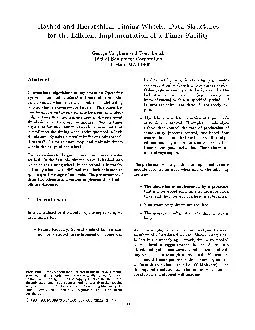
and Hierarchical Timing Wheels: Data Structures for the Efficient Impl - PDF document

and Hierarchical Timing Wheels: Data Structures for the Efficient Implementation of a Timer Facility Varghese and Tony Lauck Digital Equipment Corporation Littleton, MA 01460 algorithms to implement an Operating System timer module take to start or main- rain a timer, where n is the number of outstanding timers: this is expensive for large n. This paper be- Two 1 Introduction In a centralized or distributed operating • Failure Recovery: Several kinds of failures can- not be detected asynchronously. Some can to copy without fee all or part of this material is granted provided that the copies are not made or distributed for direct commercial advantage, the ACM copyright notice and the title of the publication and its date appear, and notice is given that copying is by be detected by periodic checking (e.g. mem- ory corruption) and such timers always expire. Other failures can be only be inferred by the lack of some positive action (e.g. message ac- knowledgment) within a specified period. If failures are infrequent these Algorithms in which the notion of time or rel- ative time is integral: Examples include algo- rithms that control the rate of production of some entity (process control, rate-based flow control in communications), scheduling algo- rithms, and algorithms to control packet life- times in computer networks. These timers al- most always expire. The performance of algorithms to implement a timer module • The algorithm is implemented by a processor that is interrupted each time a hardware clock ticks, and the interrupt overhead is substantial. • Fine granularity timers are required. • The average number of outstanding timers is large. As an example, consider communications between members of a distributed system. Since messages can be lost in 25 the hardware clock interrupts the host every tick, and the interval between ticks is in the order of mi- croseconds, then the interrupt overhead is substan- tial. Most host operating systems offer timers of coarse (milliseconds or seconds) granularity. Alter- nately, in some systems finer granularity timers re- side in special purpose hardware. In either case, the performance of the timer algorithms will be an issue as they determine the latency incurred in starting or stopping a timer and the number of timers that can be simultaneously outstanding. 2 Model and Performance Measures Our model of a timer module has four component routines: START_TIMER(Interval, Request_ID, Expiry_ Action): The client calls this routine to start a timer that will expire after "Interval" units of time. The client supplies a Request_ID which is used to distin- guish this timer from other timers that the client has outstanding. Finally, the client can specify what ac- tion must be taken on expiry: for instance, calling a client-specified routine, or setting an event flag. STOP_TIMER(Request_ID): This routine uses its knowledge of the client and Request_ID to locate the timer and stop it. PER_TICK_BOOKKEEPING: Let the granularity of the timer-be T units. Then every T units this routine checks whether any outstanding timers have expired; if so, it calls STOP_TIMER, which in turn calls the next routine. EXPIRY_PROCESSING: This routine does the Ex- piry_Action specified in the START_TIMER call. The first two routines are activated on client calls while the last two are invoked on timer ticks. The timer is often an external hardware clock. The following two performance measures can be used to choose between the various algorithms described in the rest of this paper. Both of them are parame- terized by n, the average (or worst-case) number of outstanding timers. 1. SPACE: The memory required for the data structures used by the timer module. 2. LATENCY: The time between the invoking of a routine in the timer module and its completion, assuming that the caller of the routine blocks until the routine completes. Both the average and worst case latency are of interest. For example, a client application that implements a transport protocol may find that space is cheap and the critical parameters for each routine in the timer module are as shown in Figure 1. The performance measures important for the client applications should be used to choose among timer algorithms. 3 Currently Used Timer Schemes There are two schemes we know of: Scheme 1 -- Here 3 START_TIMER finds a memory location and sets that location to the specified timer interval. Ev- ery T units, PER_TICK_BOOKKEEPING will decre- ment each outstanding timer; if any timer becomes zero, EXPIRY_PROCESSING is called. This scheme is extremely fast for all but PER_TICK_BOOKKEEPING. It also uses one record per outstanding timer, the minimum space possible. Its performance is summarized in Figure 4. It is appropriate if: * there are only a few outstanding timers. • most timers are stopped within a few ticks of the clock. • PER_TICK_PROCESSING is done with suit- able performance by special-purpose hardware. Note that instead of doing a DECREMENT, we can store the absolute time at which timers expire and do a COMPARE. This option is valid for all timer schemes we describe; the choice between them will depend on the size of the time-of-day field, the cost of each instruction, and the hardware on the machine implementing these algorithms. In this paper we will use the DECREMENT option, except when describ- ing Scheme 2. 25 Scheme 2 -- ORDERED LIST/TIMER QUEUES 3 PER_TICK_BOOKKEEPING latency is re- duced at the expense of START_TIMER. Timers are stored ill an ordered list. Unlike Scheme 1, we will store the absolute time at which the timer expires, and not the interval before expiry. The timer that is due to expire at the earliest time is stored at the head of the list. Subsequent timers are stored in increasing order as shown in Figure 2. In Fig. 2 the lowest timer is due to expire at absolute time 10 hours, 23 minutes, and 12 seconds. Because the list is sorted, PER_TICK_PROCESSING need only increment the current time of day, and com- pare it with the head of the list. If they are equal, or the time of day is greater, it deletes that list ele- ment and calls EXPIRY_PROCESSING. It continues to delete elements at the head of the list until the expiry time of the head of the list is strictly less than tile time of day. START_TIMER searches the list to find the po- sition to insert the new timer. In the example, START_TIMER will insert a new timer due to expire at 10:24:01 between the second and third elements. The worst case latency to start a timer is average latency depends on the distribution of timer intervals (from time started to time stopped), and the distribution of the arrival process according to which calls to START_TIMER are made. Interestingly, this can be modeled (Figure 3) as a sin- gle queue with infinite servers; this is valid because every timer in the queue is essentially decremented (or served) every timer tick. It is shown in I4 that we can use Little's result to obtain the average number in the queue; also the distribution of the remaining time of elements in the timer queue seen by a new re- quest is the residual life density of the timer interval distribution. If the arrival distribution is Poisson, the list is searched from the head, and reads and writes both cost one unit, then the average cost of insertion for negative exponential and uniform timer interval dis- tributions is shown in 4 to be: + 2/3n -- exponential + 1/2n -- Results for other timer interval distributions can be computed using a result in 4. For a negative expo- nential distribution we can reduce the average cost to + n/3 searching the list from the rear. In fact, if timers are always inserted at the rear of the list, this search strategy yields an O(1) START_TIMER latency. This happens, for instance, if all timers in- tervals have the same value. However, for a get---1 distribution of the timer interval, we assume the av- erage latency of insertion is need not search the list if the list is doubly linked. When START_TIMER inserts a timer into the ordered list it can store a pointer to the element. STOP_TIMER can then use this pointer to delete the element in O(1) time from the doubly linked list. This can be used by any timer scheme. If Scheme 2 is implemented by a host processor, the interrupt overhead on every tick can be avoided if there is hardware support to maintain a single timer. The hardware timer is set to expire at the time at which the the timer at the head of the list is due to expire. The hardware intercepts all clock ticks and interrupts the host only when a timer actually expires. Unfortunately, some processor architectures do not offer this capability. Algorithms similar to Scheme 2 are used by both VMS and UNIX in implementing their timer modules. The performance of the two schemes is summarized in Figure 4. As for Space, Scheme 1 needs the minimum space possible; Scheme 2 needs space for the forward and back pointers between queue elements. Timer Algorithms, Sorting Tech- niques, and Time-Flow Mecha- nisms in Discrete Event Simula- tions Sorting Algorithms and Priority Queues Scheme 2 reduced PER_TICK_BOOKKEEPING la- tency at the expense of START_TIMER by keeping the timer list sorted. Consider the relationship be- tween timer and sorting algorithms depicted in Figure 5. However: • In a typical sort all elements are input to the 27 when the sort begins; the sort ends by outputting all elements in sorted order. A timer module performs a more dynamic sort because elements arrive at different times and are out- put at different times. In a timer module, the elements to be "sorted" change their value over time if we store the in- terval. This is not true if we store the absolute time of expiry. A data structure that allows "dynamic" sorting is a priority queue 5. A priority queue allows elements to be inserted and deleted; it also allows the smallest ele- ment in the set to be found. A timer module can use a priority queue, and do PER_TICK_BOOKKEEPING only on the smallest timer element. Scheme 3: Tree-based Algorithms linked list (Scheme 2) is one way of implement- ing a priority queue. For large n, tree-based data structures are better. These include unbalanced bi- nary trees, heaps, post-order and end-order trees, and leftist-trees 4,6. They attempt to reduce the la- tency in Scheme 2 for START_TIMER from O(n) to 7 it is reported that this difference is significant for large n, and that unbalanced binary trees are less expensive than balanced binary trees. Unfortunately, unbalanced binary trees easily degen- erate into a linear llst; this can happen, for instance, if a set of equal timer intervals are inserted. We will lump these algorithms together as Scheme 3: Tree-based algorithms. The performance of Scheme 3 is summarized in Figure 6. Discrete Event Simulation discrete event simulations 8, all state changes in the system take place at discrete points in time. An important part of such simulations are the event- handling routines or time-flow mechanisms. When an event occurs in a simulation, it may schedule future events. These events are inserted into some list of outstanding events. The simulation proceeds by pro- cessing the earliest event, which in turn may sched- ule further events. The simulation continues until the event list is empty or some condition (e.g. clock � MAX-SIMULATION-TIME} holds. There are two ways to find the earliest event and up- date the clock: 1. 2. The earliest event is immediately retrieved from some data structure {e.g. a priority queue 5) and the clock jumps to the time of this event. This is embodied in simulation languages like GPSS 9 and SIMULA 10. In the simulation of digital circuits, it is often sufficient to consider event scheduling at time instants that are multiples of the clock inter- val, say c. Then, after the program processes an event, it increments the clock variable by c until it finds any outstanding events at the cur- rent time. It then executes the event(s). This is embodied in languages for digital simulation like TEGAS Ill and DECSIM 12. We have already seen that algorithms used to im- plement the first method are applicable for timer al- gorithms: these include linked lists and tree-based structures. What is more interesting is that algo- rithms for the second method are also applicable. Translated in terms of timers, the second method for PER_TICK_BOOKKEEPING is: "Increment the clock by the clock tick. If any timer has expired, call EXPIRY_PROCESSING." An efficient and widely used method to implement the second method is the so-called timing-wheel 11,13 technique. In this method, the data structure into which timers are inserted is an array of lists, with a single overflow list for timers beyond the range of the array. In Figure 7, time is divided into cycles; each cycle is N units of time. Let the current number of cycles be S. If the current time pointer points to element i, the current time is S * N + i. The event notice corresponding to an event scheduled to arrive within the current cycle (e.g. at time S * N + j, for integer j between 0 and n) is inserted into the list pointed to by the jth element of the array. Any event occurring beyond the current cycle is inserted into the overflow list. Within a cycle, the simulation increments the current time until it finds a non-empty list; it then removes and processes all events in the list. If these schedule future events within the current cycle, such events are inserted into the array of lists; if not, the new events are inserted into the overflow list. The current time pointer is incremented modulo N. When it wraps to 0, the number of cycles is incre- mented, and the overflow list is checked; any elements due to occur in the current cycle are removed from the overflow list and inserted into the array of lists. This is implemented in TEGAS-2 Ill. 28 array can be conceptually thought of as a timing wheel; every time we step through N locations, we ro- tate the wheel by incrementing the number of cycles. A problem with this implementation is that as time increases within a cycle and we travel down the ar- ray it becomes more likely that event records will be inserted in the overflow list. Other implementations 12 reduce (but do not completely avoid) this effect by rotating the wheel half-way through the array. In summary, we note that time flow algorithms used for digital simulation can be used to implement timer algorithms; conversely, timer algorithms can be used to implement time flow mechanisms in simulations. However, there are differences to note: • In Digital Simulations, most events happen within a short interval beyond the current time. Since timing wheel implementations rarely place event notices in the overflow list, they do not optimize this case. This is not true for a general purpose timer facility. • Most simulations ensure that if 2 events are scheduled to occur at the same time, they are removed in FIFO order. Timer modules need not meet this restriction. • Stepping through empty buckets on the wheel represents overhead for a Digital Simulation. In a timer module we have to increment the clock anyway on every tick. Consequently, stepping through empty buckets on a clock tick does not represent significant extra overhead is done by the same entity that maintains the current time. • Simulation Languages assume that canceling event notices is very rare. If this is so, it is suffi- cient to mark the notice as "Canceled" and wait until the event is scheduled; at that point the scheduler discards the event. In a timer module, STOP_TIMER may be called frequently; such an approach can cause the memory needs to grow unboundedly beyond the number of timers outstanding at any time. We will use the timing-wheel method below as a point of departure to describe further timer algorithms. 4 -- Basic Scheme for Timer Intervals within a Specified Range describe a simple modification of the timing wheel If we can guarantee that all timers for periods less than modified algorithm takes O(1} latency for START_TIMER, STOP_TIMER, and PER_TICK_BOOKKEEPING. Let the granularity of the timer be 1 unit. The cur- rent time is represented in Figure 8 by a pointer to an element in a circular buffer with dimensions 0, - To set a timer at j units past current time, we in- dex (Figure 8) into Element put the timer at the head of a list of timers that will expire at a time = ÷ j Each tick we increment the current timer pointer check the array element be- ing pointed to. If the element is 0 (no list of timers waiting to expire), no more work is done on that timer tick. But if it is non-zero, we do EX- PIRY_PROCESSING on all timers that are stored in that list. Thus the latency for START_TIMER is O(1); PER_TICK_BOOKKEEPING is O(1) except when timers expire, but we can't do better than that. If the timer lists are doubly linked, and, as before, we store a pointer to each timer record, then the latency of STOP_TIMER is also O(1). This is basically a timing wheel scheme where the wheel turns one array element every timer unit, as opposed to rotating every 11. This guarantees that all timers within the current time will be inserted in the array of lists; this is not guaranteed by conventional timing wheel algorithms 11,13. In sorting terms, this is a bucket sort 5,14 that trades off memory for processing. However, since the timers change value every time instant, intervals are entered as offsets from the current time pointer. It is sufficient if the current time pointer increases every time instant. A bucket sort sorts N elements in using M buckets, since all buckets have to be examined. This is inefficient for large M � N. In timer algo- rithms, however, the crucial observation is that some entity needs to do O(1) work per tick to update the current time; it costs only a few more instructions for the same entity to step through an empty bucket. What matters, unlike the sort, is not the total amount 29 using this larger values array using the table size bitrary size (low order pointer to result of table size 8 bits. order bits inserted into a are possible. choice at are two with Sorted the correct n i - - Since i n O(1). How the arrival pointer. If as in scheme reduces insertion sort sort on the lists pointed to by each bucket. 6.1.2 Scheme 6: Hash Table with Unsorted of O(1). as in has the list will of how average per n on average timers hash into ticks we do O(1) work. Thus the hash distribution in Scheme 6 only con- trols the ~burstiness" (variance) of the latency of PER_TICKBOOKKEEPING, and not the average latency. Since the worst-case latency of PER_TICK_- BOOKKEEPING is always timers expire at the same time), we believe that that the choice of hash function for Scheme 6 is insignificant. Obtain- ing the remainder after dividing by a power of 2 is cheap (AND instruction), and consequently recom- mended. Further, using an arbitrary hash function to map a timer value into an array index would re- quire PER_TICK_BOOKKEEPING to compute the hash on each timer tick, which would make it more expensive. We discuss implementation strategies for Scheme 6 in Appendix A. Extension 2: Exploiting Hierarchy, Scheme 7 last extension of the basic scheme exploits the concept of hierarchy. To represent the number 1000000 we need only 7 digits instead of 1000000 be- cause we represent numbers hierarchically in units of l's, 10's, 100's etc. Similarly, to represent all possible timer values within a 32 bit range, we do not need a 222 element array. Instead we can use a number of arrays, each of different granularity. For instance, we can use 4 arrays as follows: A 100 element array in which each element rep- resents a day A 24 element array in which each element rep- resents an hour A 60 element array in which each element rep- resents a minute A 60 element array in which each element rep- resents a second Thus instead of 100 * 24 * 60 * 60 = 8.64 million locations to store timers up to 100 days, we need only 100 + 24 + 60 + 60 = 244 locations. As an example, consider Figure 10. Let the current time be 11 days 10 hours, 24 minutes, 30 seconds. Then to set a timer of 50 minutes and 45 seconds, we first calculate the absolute time at which the timer will expire. This is 11 days, 11 hours, 15 minutes, 15 seconds. Then we insert the timer into a list begin- ning 1 (11 - 10 hours) element ahead of the current hour pointer in the hour array. We also store the remainder (15 minutes and 15 seconds) in this loca- tion. We show this in Figure 10, ignoring the day array which does not change during the example. The seconds array works as usual: every time the hardware clock ticks we increment the second pointer. If the list pointed to by the element is non-empty, we do EXPIRY_PROCESSING for elements in that list. However, the other 3 arrays work slightly differently. Even if there are no timers requested by the user of the service, there will always be a 60 second timer that is used to update the minute array, a 60 minute timer to update the hour array, and a 24 hour timer to update the day array. For instance, every time the 60 second timer expires, we will in- crement the current minute timer, do any required EXPIRY_PROCESSING for the minute timers, and re-insert another 60 second timer. Returning to the example, ff the timer is not stopped, eventually the hour timer will reach 11. When the hour timer reaches 11, the list is examined; EX- PIRY_PROCESSING will insert the remainder of the seconds (15) in the minute array, 15 elements after the current minute pointer(0). Of course, if the min- utes remaining were zero, we could go directly to the second array. At this point, the table will look like Figure 11. Eventually, the minute array will reach the 15th el- ement; as part of EXPIRY_PROCESSING we will move the timer into the SECOND array 15 seconds after the current value. 15 seconds later the timer will actually expire, and we do the user-specified EX- PIRY_PROCESSING. What are the performance parameters of this scheme? START_TIMER: Depending on the algorithm, we may need 0(rn) time, where m is the number of arrays in the hierarchy, to find the right table to insert the timer and to find the remaining time. A small num- ber of levels should be sufficient to cover the timer range with an allowable amount of memory; thus m should be small (2 _rn 5 say.) STOP_TIMER: Once again this can be done in O(1) time if all lists are doubly linked. PER_TICK_BOOKKEEPING: It is useful to com- pare this to the corresponding value in Scheme 6. 31 have the same average latency of O(I) for suf- ficiently large array sizes but the constants of com- plexity are different. More precisely: let T be the average timer interval (from start to stop or expiry). Let M be the total amount of array elements avail- able. Let m be the total number of levels in the hierarchy. The total work done in Scheme 6 for such an average sized timer is: T/M where c(6) is a constant denoting the cost of decre- menting the high order bits, indexing etc. in Scheme 6. If a timer lives for T units of time, it will be decre- mented T/M times. And in Scheme 7 it is bounded from above by: c(7) * m where c(7) represents the cost of finding the next list to migrate to, and the cost of migration, in Scheme 7; m is the maximum number of lists to migrate be- tween. The average cost per unit time for an average of n timers then becomes: c(6) Scheme 6 n * c(7) * m / W Scheme 7 The choice between Scheme 6 and Scheme 7 will de- pend on the parameters above. Since c(6) and c(7) will not be drastically different, for small values of T and large values of M, Scheme 6 can be better than Scheme 7 for both START_TIMER and PER_TICK-- BOOKKEEPING. However, for large values of T and small values of M, Scheme 7 will have a better aver- age cost (latency) for PER_TICK_BOOKKEEPING but a greater cost for START_TIMER. Wick Nichols has pointed out that ff the timer pre- cision is allowed to decrease with increasing levels in the hierarchy, then we need not migrate timers be- tween levels. For instance, in the example above we would round off to the nearest hour and only set the timer in hours. When the hour timer goes off, we do the user specified EXPIRY_PROCESSING without migrating to the minute array. Essentially, we now have different timer modes, one for hour timers, one for minute timers, etc. This reduces PER_TICK_- BOOKKEEPING overhead further at the cost of a in precision of up to 50% (e.g. a 1 minute and 30 second timer that is rounded to 1 minute). Alter- nately, we can improve the precision by allowing just one migration between adjacent lists. Scheme 7 has an obvious analogy to a radix sort 5,14. We discuss implementation strategies for Scheme 7 in Appendix A. Summary and Conclusions this paper, we have examined the relationship be- tween sorting algorithms, time flow mechanisms in event simulations, and timer algorithms. We have extended the timing wheel mechanism used in logic simulation to yield 3 timer algorithms (Schemes 5-7) that have constant complexity for setting, stop- ping, and maintaining a timer. The extensions in- clude rotating the timing wheel every clock tick, hav- ing separate overflow lists per bucket, and using a hierarchical set of timing wheels (Scheme 7): the ex- tensions are necessary because the requirements of a scheduler in a logic simulation and those of a general timer module are different. In choosing between schemes, we believe that Scheme 1 is appropriate in some cases because of its simplic- ity, limited use of memory, and speed in starting and stopping timers. Scheme 2 is useful in a host that has hardware to maintain the clock and a single timer. Although it takes O(n) time to start a timer, tlle host is not interrupted every clock tick. In a host (e.g. a VAX) without hardware support for timers, we believe Schemes 2 and 3 are inappropriate because of the cost of START_TIMER when there are a large number of outstanding timers. Clearly, this is not uncommon in hosts that have a signifi- cant amount of real-time activity or have several open communication links. Scheme 4 is useful when most timers are within a small range of the current time. For example, it could be used by a networking module that is maintaining its own timers. Scheme 5 depends too much on the hash distribution (for a fast START_TIMER) to be generally useful. For a general timer module, similar to the operating system facilities found in UNIX or VMS, that is ex- pected to work well in a variety of environments, we recommend Scheme 6 or 7. We have implemented Scheme 6 on a VAX using 32 We used cheap VAX instructions, where the average cost of a "cheap" instruction can be taken to be that of a CLRL (longword clear). We did not use VAX Queue instructions. The numbers given below for the implementation do not include the cost of synchronization (e.g. by lowering and rais- ing interrupt priority levels) in the START_TIMER and STOP_TIMER routines; they are needed for any timer algorithm and their costs are machine specific. Tile implementation took 13 cheap VAX instructions to insert a timer and 7 to delete a timer. The cost per tick was 4 instructions to skip an empty array lo- cation, and 6 instructions to decrement a timer and move to the next queue element. A further 9 instruc- tions were needed to delete an expired timer and call the EXPIRY_PROCESSING routine. Thus even if we assume that every outstanding timer expires dur- ing one scan of the table, the average cost per tick is 4 + 15 * n/TableSize instructions. {Once again this is because during every scan of the table all n --the average number of outstanding timers -- timers will be decremented and possibly expire.) If the size of the array is much larger than rt, the average cost per tick can be close to 4 instructions. If the amount of memory required for an efficient im- plementation of Scheme 6 is a problem, Scheme 7 can be pressed into service. Scheme 7, however, will need a few more instructions in START_TIMER to find the correct table to insert the timer. Both Schemes 6 and 7 can be completely or partially (see Appendix A) implemented in hardware using some auxiliary memory to store the data structures. If a host had such hardware support, the host soft- ware would need O(1} time to start and stop a timer and would not need to be interrupted every clock tick. Finally we note that designers and implementors have assumed that protocols that use a large number of timers are expensive and perform poorly. This is an artifact of existing implementations and operat- ing system facilities. Given that a large number of timers can be implemented efficiently {e.g. 4 to 13 VAX Instructions to start, stop, and, on the aver- age, to maintain timers), we hope this will no longer be an issue in the design of protocols for distributed systems. 8 Acknowledgments Barry Spinney suggested extending Scheme 4 to Scheme 5. Hugh Wilkinson independently thought of exploiting hierarchy in maintaining timer lists. John Forecast helped us implement Scheme 6. Andrew Black commented on an earlier version and helped improve the presentation. Andrew Black, Barry Spin- hey, Hugh Wilkinson, Steve Glaser, Wick Nichols, Paul Koning, Alan Kirby, Mark Kempf, and Char- lie Kaufman {all at DEC) were a pleasure to discuss these schemes with. We would like to thank Ellen Gilliam for her help in assembling the references, and the program committee for helpful comments. 9 References 1. N.P. Kronenberg, H. Levy, W.D. Strecker,, "VAXclusters: A Closely- Coupled Distributed System," ACM Trans. on Computer Systems, Vol. 4, No., May 1986, 2. A.S. Tanenbaum and R. van Renesse, "Dis- tributed Operating Systems," Computing Sur- veys, Vol. 17, No. 4, December 1985 3. A.S. Tanenbaum, "Computer Net- works," Prentice-Hall, Englewood Cliffs, N.J., 1981. Reeves, "Complexity Analysis of Event Set Algorithms," Computer Journal, Vol. 27, no. 1, 1984 5. D.E. Knuth, "The Art of Computer Program- ming, Volume 3," Addison Wesley, Reading, MA 1973. 6. J.G. Vaucher and P. Duval, "A Comparison Of Simulation Event List Algorithms," CACM 18, 1975. 7. B. Myhrhaug, "Sequencing Set Efficiency," Pub. A9, Norwegian Computing Centre, Fork- sningveien, 1B, Oslo 3. Pritsker, P.J. Kiviat, "Simulation with GASP-II," Prentice-Hall, Englewood Cliffs, N.J., 1969.. . "General Purpose Simulation System 360- User's Manual," Pub. H20-0326, IBM Corp., White Plains, N.Y., 1968. 33 11. 12. 13. 14. O-J Dahl, B. Myhrhaug,and K. Nygaard, "SIM- ULA 67 Common Base Language," Pub. $22 Norwegian Computing Centre, Forksningveien, 1B, Oslo 3. S. Szygenda, C.W. Hemming, and J.M. Hemphill, "Time Flow Mechanisms for use in Digital Logic Simulations," Proc. 1971 Winter Simulation Conference, New York. M.A. Kearney, "DECSIM: A Multi-Level Sim- ulation System for Digital Design," 1984 Inter- national Conference on Computer Design. Ulrich, "Time-Sequenced Logical Simulation Based on Circuit Delay and Selective Tracing of Active Network Paths," 1965 ACM National Conference. A. Aho, J. Hopcoft, J. Ullman, "The Design and Analysis of Computer Algorithms, "Addi- son Wesley, Reading, MA, 1974 Implementation Considerations A.1 Hardware Assist Since the cost of handling clock interrupts becomes more significant for fine granularity (e.g. microsec- onds) timers, it may be necessary to employ special purpose hardware assist. In the extreme, we can use a timer chip which maintains all the data structures (say in Scheme 6) and interrupts host software only when a timer expires. possibility is a chip (actually just a counter) that steps through the timer arrays, and interrupts the host only if there is work to be done. When the host inserts a timer into an empty queue pointed to by array element X it tells the chip about this new queue. The chip then marks X as "busy". As before, the chip scans through the timer arrays every clock tick. During its scan, when the chip encounters a "busy" location, it interrupts the host and gives the host the address of the queue that needs to be worked on. Similarly when the host deletes a timer entry from some queue and leaves behind an empty queue it needs to inform the chip that the corresponding array location is no longer "busy". Note that the synchronization overhead is minimal because the host can keep the actual timer queues in its memory which the chip need not access, and the chip can keep the timing arrays in its memory, which the host need not access. The only communication between the host and chip is through interrupts. In Scheme 6, the host is interrupted an average of per timer interval, where T is the aver- age timer interval and M is the number of array ele- ments. In Scheme 7, the host is interrupted at most m times, where m is the number of levels in the hi- erarchy. If T and m are small and M is large, the interrupt overhead for such an implementation can be made negligible. we note that conventional hardware timer chips use Scheme 1 to maintain a small number of timers. However, if Schemes 6 and 7 are imphmented a single chip that operates on a separate memory (that contains the data structures) then there is no a priori limit on the number of timers that can be handled by the chip. Clearly the array sizes need to be parameters that must be supplied to the chip on initialization. Symmetric Multiprocessing If the host consists of a set of processors, each of which can process calls to the timer module (sym- metric multiprocessing), Steve Glaser has pointed out that algorithms that tie up a common data struc- ture for a large period of time will reduce efficiency. For instance in Scheme 2, when Processor A inserts a timer into the ordered list other processors cannot process timer module routines until Processor A fin- ishes and releases its semaphore. Scheme 5, 6, and 7 seem suited for implementation in symmetric multi- processors. STA RT_TI M E R STOP_TIMER PERTICKBOOKKEEPING EXPIRY_PROCESSING CRITICAL PARAM ETER LATENCY LATENCY LATENCY NONE 1 - AN EXAMPLE OF THE PARAMETERS OF THE TIMER MODULE THAT A NETWORKING APPLICATION MIGHT CONSIDER IMPORTANT I., ..m ._m "t 10:23"24 I. 10:24:03 r I I" "l queue head 2 - TIMER QUEUE EXAMPLE USED TO ILLUSTRATE SCHEME 2 to I timer module /'x with pdfa(t) .. servers, service pdf = s(t) Expired or stopped timers Note: s(t) is density function of interval between starting and stopping (or expiration) of a timer 3 - A G/G/INF/INF QUEUEING MODEL OF A TIMER MODULE 1 Scheme 2 STA RT_TI M ER LATENCY 0(1) O(n) STOP_TIM PER_TICK_BOOKKEEPING LATENCY O(n) 0(1) 4- COMPARING AVERAGE AND WORST-CASE LATENCIES OF SCHEMES 1 AND 2 of unsorted Timer Requests _1 TIMER MODULE I (SORTING MODULE) I in sorted order (ignoring stopped timers) 5 - ANALOGY BETWEEN ATIMER AND A SORTING MODULE RT_TI M E R LATE NCY O(Iog(n)) STOP_TIMER LATENCY 0(1) or O(Iog(n)) PER_TICKBOOKKEEPING LATENCY STOP_TIMER is O(1) for unbalanced trees and O(Iog(n)) --- because of the need to rebalance the tree after a deletion --- for balanced trees 6 - AVERAGE LATENCY FOR TREE-BASED SCHEMES 0 Element 1 Element i Elementj Element N-1 0 0 0 0 Current Time List of timers to expire at this time I NU mber of Cycles J Overflow List 7 - TIMING WHEEL MECHANISM USED IN LOGIC SIMULATION 11 0 Element I Element i Element i + j Element Maxlnterval -1 0 0 0 Current Time List of timersto expire at this time 8-ARRAYOF LISTS USED BY SCHEME 4 FOR TIMER INTERVALS UP TO A MAXIMUM INTERVAL 0 Element 1 Element 10 Element 30 Element 255 0 0 0 4 0 Current Time List of timers that have hashed into this bucket 9-ARRAYOF LISTS USED BY SCHEMES 5 AND 6 FOR ARBITRARY SIZED TIMERS: BASICALLY A HASH TABLE ARRAY MINUTE ARRAY SECOND ARRAY Current Hour Pointer = 10 Current minute Pointer = 24 Current second Pointer = 30 I Timer Record with Remaining Time = 15 minutes, 15 seconds I FIGURE 10 - HIERARCHICAL SET OF ARRAYS USED BY SCHEME 7 TO "MAP" TIME MORE EFFICIENTLY HOUR ARRAY MINUTE ARRAY SECOND ARRAY Current minute Current second Pointer = 0 �--- Pointer = 0 �--- Current Hour Pointer = 11 Element 15 T Record with Remaining Time = 15 seconds I FIGURE 11 - FIGURE 10 AFTER THE HOUR COMPONENT EXPIRES 38