
McGrawHillIrwin Copyright 2011 by the McGrawHill Companies Inc All rights reserved Elasticity Issue How responsive is the demand for goods and services to changes in prices ceteris paribus The concept of price elasticity of demand is useful here ID: 273052
Download Presentation The PPT/PDF document "Chapter 6: Elasticity and Demand" is the property of its rightful owner. Permission is granted to download and print the materials on this web site for personal, non-commercial use only, and to display it on your personal computer provided you do not modify the materials and that you retain all copyright notices contained in the materials. By downloading content from our website, you accept the terms of this agreement.


Slide1
Chapter 6: Elasticity and Demand
McGraw-Hill/Irwin
Copyright © 2011 by the McGraw-Hill Companies, Inc. All rights reserved.Slide2
Elasticity
Issue: How responsive is the demand for
goods and services to
changes in
prices,
ceteris paribus. The concept of price elasticity of demand is useful here.Slide3
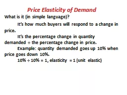
Price elasticity of demand
Let price elasticity of demand (E
P
) be given by:
E
P
=
% change in Q
% change in P
[1
]Slide4
Price
0
Output
P = 290 – Q/2
240
235
100
110
Question: What is E
P
in the range of demand curve between
prices of
$240 to $235? To find out:
Meaning, a 1% increase in
prices will
result in a 4.8%
decrease
in
quantity-demanded (and
vice-versa).
A
BSlide5
Point elasticity
In our previous example we computed the elasticity for a certain segment of the demand curve (point A to B). For purposes of marginal analysis, we are interested in point elasticity—meaning, elasticity when the change in price in infinitesimally small.Slide6
Formula for point elasticity
[2]
Here we are calculating the responsiveness of sales to a change in price
at
a point on the demand curve—that is, a defined price-quantity point .Slide7
Arc elasticity
To compute arc elasticity, or “average” elasticity between two price-quantity points on the demand curve:
N
ote
the advantage of arc elasticity—that is, it matters
not
what the initial price is (say, $240 or $235), our calculation of E
P
does not change.Slide8
Elasticity
Responsiveness
E
Elastic
Unitary Elastic
Inelastic
Table 6.1
Price Elasticity of Demand (
E
)
%
∆
Q
>
%
∆
P
%
∆
Q
=
%
∆
P
%∆
Q< %∆P
E> 1
E
= 1
E
< 1Slide9
Factors Affecting Price Elasticity of Demand
Availability of substitutes The better & more numerous the substitutes for a good, the more elastic is demandPercentage of consumer’s budget
The greater the percentage of the consumer’s budget spent on the good, the more elastic is demand
Time period of adjustment
The longer the time period consumers have to adjust to price changes, the more elastic is demandSlide10
Perfectly inelastic demand
P
r
i
c
e
5
0
Q
u
a
n
t
i
t
y
1
0
0
1
5
0
2
0
0
2
5
0
1
0
3
0
2
0
5
0
4
0
7
0
6
0
8
0
9
0
$
1
0
0
E
P
=
0
0
Buyers are absolutely non-responsive to a change in priceSlide11
Perfectly elastic demand
E
P
=
- infinity
P
r
i
c
e
5
0
Q
u
a
n
t
i
t
y
1
0
0
1
5
0
2
0
0
2
5
0
1
3
2
5
4
7
6
8
9
$
1
0
(
b
)
P
e
r
f
e
c
t
l
y
E
l
a
s
t
i
c
D
e
m
a
n
d
0
In this case, if the price rises a penny above $5, quantity-demanded falls to zero.Slide12
Price Elasticity Changes Along a Linear Demand Curve
$
4
0
0
3
0
0
2
0
0
1
0
0
4
0
0
1
,
2
0
0
,
1
6
0
0
Q
u
a
n
t
i
t
y
D
e
m
a
n
d
e
d
P
r
i
c
e
8
0
0
M
a
r
g
i
n
a
l
r
e
v
e
n
u
e
D
e
m
a
n
d
i
s
p
r
i
c
e
e
l
a
s
t
i
c
D
e
m
a
n
d
i
s
p
r
i
c
e
i
n
e
l
a
s
t
i
c
B
M
A
E
l
a
s
t
i
c
i
t
y
=
-1
M
R
=
4
0
0
-
.
5
Q
P
=
4
0
0
-
.
2
5
Q
0
(
a
)
Demand tends to be elastic at higher prices and inelastic at lower pricesSlide13
Constant Elasticity of Demand
(Figure 6.3)Slide14
Check Station
Prove that price elasticity is unity at point M
Therefore :Slide15
Income Elasticity
Income elasticity (EM) measures the responsiveness of quantity demanded to changes in income, holding the price of the good & all other demand determinants constant
Positive for a normal good
Negative for an inferior goodSlide16
Cross price elasticity of demand
How sensitive is the demand for rental cars to airline fares?
How does the demand for apples respond to a change in the price of oranges?
Will a strong dollar hurt tourism in Florida?
Cross price elasticity gives us a measure of the responsiveness of demand to the price of complements or substitutesSlide17
Cross-Price Elasticity
Cross-price elasticity (EXR) measures the responsiveness of quantity demanded of good
X
to changes in the price of related good
R
, holding the price of good
X
& all other demand determinants for good X constantPositive when the two goods are substitutesNegative when the two goods are complementsSlide18
Revenue rule
Revenue rule:
When demand is elastic, price and revenue move inversely. When demand is inelastic, price and revenue move together.
As price falls along the
elastic
portion of the demand curve (price above $200), revenue will increase; whereas as price falls along the inelastic portion (below $200), revenue will decreaseSlide19
Marginal Revenue
Marginal revenue (MR) is the change in total revenue per unit change in outputSince MR
measures the rate of change in total revenue as quantity changes,
MR
is the slope of the total revenue
(
TR
) curve Slide20
Unit sales (Q)
Price
TR = P
Q
MR =
TR/Q
0
$4.50
1
4.00
2
3.50
3
3.10
4
2.80
5
2.40
6
2.00
7
1.50
Demand & Marginal Revenue
(Table 6.3)
$ 0
$
4.00
$
7.00
$
9.30
$
11.20
$
12.00
$
12.00
$
10.50
--
$4.00
$
3.00
$
2.30
$
1.90
$
0.80
$
0
$
-1.50
Slide21
Demand,
MR, & TR (Figure 6.4)
Panel A
Panel BSlide22
Demand & Marginal Revenue
When inverse demand is linear, P = A + BQ (A > 0, B < 0)Marginal revenue is also linear, intersects the vertical (price) axis at the same point as demand, & is twice as steep as demand
MR = A + 2BQSlide23
Linear Demand,
MR, & Elasticity (Figure 6.5)Slide24
Marginal Revenue & Price Elasticity
For all demand & marginal revenue curves, the relation between marginal revenue, price, & elasticity can be expressed asSlide25
$
1
6
0
,
0
0
0
1
2
0
,
0
0
0
4
0
0
1
,
2
0
0
Q
u
a
n
t
i
t
y
D
e
m
a
n
d
e
d
R
e
v
e
n
u
e
8
0
0
(
b
)
T
o
t
a
l
r
e
v
e
n
u
e
R
=
4
0
0
Q
-
.
2
5
Q
2
0
Notice the Marginal Revenue (MR) function dips below the horizontal axis at Q = 800. Slide26
Price Elasticity & Total Revenue
Elastic
Quantity-effect dominates
Unitary elastic
No dominant effect
Inelastic
Price-effect dominates
Price rises
Price falls
TR
falls
TR
rises
No change in
TR
No change in
TR
TR
rises
TR
falls
Table 6.2
%
∆
Q
>
%∆P %∆Q= %∆P
%∆Q< %∆P Slide27
Check Station
The management of a professional sports team has a 36,000-seat stadium it wishes to fill. It recognizes, however, that the number of seats sold (Q) is very sensitive to ticket prices (P). It estimates demand to be
Q = 60,000 - 3,000P
. Assuming the team’s costs are known
and do not vary with attendance
, what is the management’s optimal pricing policy?Slide28
Notice the inverse demand function is given by:
Since variable cost (and hence marginal cost) is
zero, maximizing profits means maximizing
revenue.
The revenue function is given by: