

楊立偉教授 台灣科大資管系 wyangntuedutw 本投影片修改自 Introduction to Information Retrieval 一書之投影片 Ch 6 1 Ranked Retrieval 2 3 Ranked retrieval Boolean ID: 638749
Download Presentation The PPT/PDF document "Lecture 3 : Term Weighting" is the property of its rightful owner. Permission is granted to download and print the materials on this web site for personal, non-commercial use only, and to display it on your personal computer provided you do not modify the materials and that you retain all copyright notices contained in the materials. By downloading content from our website, you accept the terms of this agreement.


Slide1
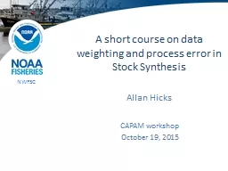
Lecture 3 : Term Weighting
楊立偉教授台灣科大資管系wyang@ntu.edu.tw本投影片修改自Introduction to Information Retrieval一書之投影片 Ch 6
1Slide2
Ranked Retrieval
2Slide3
3
Ranked
retrieval
Boolean
retrieval return d
ocuments either match or don’t.
Good for expert users
with precise understanding of their needs and of the collection.Not good for the majority of usersMost users are not capable of writing Boolean queriesMost users don’t want to go through 1000s of results.This is particularly true of web search.
3Slide4
4
Problem with Boolean search
Boolean queries often result in either too few (=0) or too
many
(1000s)
results
.
Example query : [standard user dlink 650] → 200,000 hitsExample query : [standard user dlink 650 no card found] → 0 hits
It takes a lot of skills to give a proper Boolean query.
4Slide5
5
Ranked retrieval
With ranking, large result sets are not an issue.
More relevant results are ranked higher than less relevant results
.
The user may decide how many results he/she wants.
5Slide6
6
Scoring as the basis of ranked retrieval
Assign a score to each query-document pair, say in [0, 1], to measure how well document and query “match”.
If the query term does not occur in the document: score should be 0.
The more frequent the query term in the document, the higher the score
6Slide7
7
Basic approach : using Jaccard coefficient
Example
What is the query-document match score that the
Jaccard
coefficient
computes for:Query: “ides of March”Document “Caesar died in March”JACCARD(
q, d) = 1/6
7Slide8
8
3 drawbacks of the basic approach
1. It doesn’t consider term frequency
(how many occurrences a
term
has
).2. Rare terms are more informative than frequent terms. Jaccard does not consider this information.3. Need a more sophisticated way of normalizing for the length of a document.use (cosine)
instead of |A ∩
B
|/|
A
∪
B| (
Jaccard
) for length
normalization.
8Slide9
9
Example
Cosine
Jaccard
|
A
∩
B|/|A ∪ B|9
Jaccard
favors more overlapping
than length normalization.Slide10
Term Frequency
10Slide11
11
Binary incidence
matrix
Each document is represented as a binary vector ∈ {0, 1}
|V|.
11
Anthony and CleopatraJulius Caesar
The
Tempest
Hamlet
Othello
Macbeth . . .
ANTHONY
BRUTUS
CAESAR
CALPURNIA
CLEOPATRA
MERCY
WORSER
. . .
1
1
1
0
1
1
1
1
1
1
1
0
0
0
0
0
0
0
0
1
1
0
1
1
0
0
1
1
0
0
1
0
0
1
1
1
0
1
0
0
1
0Slide12
12
Count matrix
Each document is now represented as a count vector ∈ N
|
V
|.
12
Anthony and CleopatraJulius Caesar
The TempestHamlet
Othello
Macbeth . . .
ANTHONY
BRUTUS
CAESAR
CALPURNIA
CLEOPATRA
MERCY
WORSER
. . .
157
4
232
0
57
2
2
73
157
227
10
0
0
0
0
0
0
0
0
3
1
0
2
2
0
0
8
1
0
0
1
0
0
5
1
1
0
0
0
0
8
5Slide13
13
Bag
of
words
model
Do not consider the
order of words in a document.John is quicker than Mary , and Mary is quicker than John are represented the same way.
Note: Positional index can distinguish the order.
13Slide14
14
Term frequency
tf
The term frequency
tf
t,d
of term t in document d is defined as the number of times that t occurs in d.Use tf when computing query-document match scores.
But Relevance does not increase proportionally with term frequency.
Example
A document with
tf
= 10
occurrences of the term is more relevant than a document with
tf
= 1
occurrence of the term, but not 10 times more relevant.
14Slide15
15
Log frequency weighting
The log frequency weight of term t in d is defined as follows
tf
t,d
→ w
t,d
: 0 → 0, 1 → 1, 2 → 1.3, 10 → 2, 1000 → 4, etc.Why use log ? 在數量少時, 差1即差很多;
但隨著數量越多,差
1
的影響變得越小
tf
-matching-score(
q
,
d
) =
t
∈
q
∩
d
(1 + log
tf
t
,
d
)
15Slide16
16
Exercise
Compute the
Jaccard
matching score and the
tf
matching score for the following query-document pairs.
q: [information on cars] d: “all you have ever wanted to know about cars” jaccard = 1 / 11, tf = 1+log1q: [information on cars] d: “information on trucks, information on planes, information on trains”
jaccard = 2 / 6, tf = (1+log3) + (1+log3)q: [red cars and red trucks] d: “cops stop red cars more often”
jaccard = 2 / 8, tf = (1+log1) + (1+log1)
16Slide17
TF-IDF Weighting
17Slide18
18
Frequency in document vs. Frequency in collection
In addition to term frequency (the frequency of the term in
the document)
, we also want to use the frequency of the term
in the collection
for weighting and ranking.
18Slide19
19
Desired weight for rare terms
Rare terms are more informative than frequent terms.
Consider a term in the query that is
rare
in the collection
(e.g.,
ARACHNOCENTRIC).A document containing this term is very likely to be relevant.→ We want high weights for rare terms like ARACHNOCENTRIC.
19Slide20
20
Desired weight for frequent terms
Frequent terms are less informative than rare terms.
Consider a term in the query that is
frequent
in the collection
(e.g.,
GOOD, INCREASE, LINE). → common term or 無鑑別力的詞20Slide21
21
Document
frequency
We want
high weights for rare terms
like
ARACHNOCENTRIC
.We want low (positive) weights for frequent words like GOOD, INCREASE and LINE.We will use document frequency to factor this into computing the
matching score.
The document frequency is
the number of documents in the collection that the term occurs in
.
21Slide22
22
idf
weight
df
t
is the document frequency, the number of documents that
t occurs in.dft is an inverse measure of the informativeness of term t.We define the idf
weight of term t as follows:
(
N
is the number of documents in the collection.)
idf
t
is a measure of the
informativeness
of the term.
[log
N
/
df
t
] instead of [
N
/
df
t
] to balance the effect of
idf
(i.e. use log for both
tf
and
df
)
22Slide23
23
Examples
for
idf
Compute
idf
t using the formula:23term
df
t
idf
t
calpurnia
animal
sunday
fly
under
the
1
100
1000
10,000
100,000
1,000,000
6
4
3
2
1
0Slide24
24
Collection
frequency
vs.
Document
frequency
Collection frequency of t: number of tokens of t in the collectionDocument frequency of t: number of documents t occurs inDocument/collection frequency weighting is computed from known collection, or estimated
需進行全域統計或採估計值
Which word is a more informative ?
24
word
collection
frequency
document
frequency
INSURANCE
TRY
10440
10422
3997
8760Slide25
Example
cf 出現次數 與 df 文件數。差異範例如下: Word
cf
出現總次數
df
出現文件數 ferrari 10422 17 ←較高的稀有性 (高資訊量) insurance
10440 3997Slide26
26
tf-idf
weighting
The
tf-idf
weight of a term is the
product of its
tf weight and its idf weight.tf-weight
idf-weight
Best known weighting scheme in information retrieval
Note: the “-” in
tf-idf
is a hyphen, not a minus sign
Alternative names: tf.idf , tf x idf
26Slide27
27
Summary:
tf-idf
Assign a
tf-idf
weight for each term t in each document
d
:The tf-idf weight . . .. . . increases with the number of occurrences within a document. (term
frequency). . . increases with the rarity of the term in the collection.
(inverse
document
frequency
)
27Slide28
28
Exercise: Term, collection and document frequency
Relationship between
df
and
cf
?
Relationship between tf and cf?Relationship between tf and df?28
Quantity
Symbol
Definition
term frequency
document frequency
collection frequency
tf
t,d
df
t
cf
t
number of occurrences of
t
in
d
number of documents in the
collection that
t
occurs in
total number of occurrences of
t
in
the
collectionSlide29
Vector Space Model
29Slide30
30
Binary incidence
matrix
Each document is represented as a binary vector ∈ {0, 1}
|
V
|.30Anthony and Cleopatra
Julius Caesar
The
Tempest
Hamlet
Othello
Macbeth . . .
ANTHONY
BRUTUS
CAESAR
CALPURNIA
CLEOPATRA
MERCY
WORSER
. . .
1
1
1
0
1
1
1
1
1
1
1
0
0
0
0
0
0
0
0
1
1
0
1
1
0
0
1
1
0
0
1
0
0
1
1
1
0
1
0
0
1
0Slide31
31
Count matrix
Each document is now represented as a count vector ∈ N
|
V
|.
31
Anthony and CleopatraJulius Caesar
The
Tempest
Hamlet
Othello
Macbeth . . .
ANTHONY
BRUTUS
CAESAR
CALPURNIA
CLEOPATRA
MERCY
WORSER
. . .
157
4
232
0
57
2
2
73
157
227
10
0
0
0
0
0
0
0
0
3
1
0
2
2
0
0
8
1
0
0
1
0
0
5
1
1
0
0
0
0
8
5Slide32
32
Binary → count
→
weight
matrix
Each document is now represented as a real-valued vector of
tf idf weights ∈ R|V|.32
Anthony
and
Cleopatra
Julius
Caesar
The
Tempest
Hamlet
Othello
Macbeth . . .
ANTHONY
BRUTUS
CAESAR
CALPURNIA
CLEOPATRA
MERCY
WORSER
. . .
5.25
1.21
8.59
0.0
2.85
1.51
1.37
3.18
6.10
2.54
1.54
0.0
0.0
0.0
0.0
0.0
0.0
0.0
0.0
1.90
0.11
0.0
1.0
1.51
0.0
0.0
0.12
4.15
0.0
0.0
0.25
0.0
0.0
5.25
0.25
0.35
0.0
0.0
0.0
0.0
0.88
1.95Slide33
33
Documents
as
vectors
Each document is now represented as a real-valued vector of
tf-idf
weights ∈ R|V|.So we have a |V|-dimensional real-valued vector space.Terms are axes of the space.Documents are
points or vectors in this space.
Each vector is very sparse - most entries are zero.
Very high-dimensional: tens of millions of dimensions when apply this to web (i.e. too many different terms on web)
33Slide34
34
Queries
as
vectors
Do the same for queries: represent them as vectors in the high-dimensional space
Rank documents according to their proximity to
the queryproximity = similarity ≈ negative distanceRank relevant documents higher than nonrelevant documents
34Slide35
Vector Space Model
將文件透過一組詞與其權重,將文件轉化為空間中的向量(或點),因此可以計算文件相似性或文件距離計算文件密度找出文件中心進行分群(聚類)進行分類(歸類)Slide36
Vector Space Model
假設只有Antony與Brutus兩個詞,文件可以向量表示如下D1: Antony and Cleopatra = (13.1, 3.0)D2: Julius Caesar = (11.4, 8.3)
計算文件相似性:
以向量夾角表示
用內積計算
13.1x11.4 + 3.0 x 8.3
計算文件幾何距離: Slide37
Applications of Vector Space Model
分群 (聚類) Clustering:由最相近的文件開始合併分類 (歸類
) Classification
:挑選最相近的類別
中心
Centroid
可做為群集之代表 或做為文件之主題文件密度 了解文件的分布狀況Slide38
Issues about Vector Space Model (1)
詞之間可能存有相依性,非垂直正交 (orthogonal)假設有兩詞 tornado, apple 構成的向量空間, D1=(1,0) D2=(0,1),其內積為
0
,故稱完全不相似
但當有兩詞
tornado, hurricane
構成的向量空間,
D1=(1,0) D2=(0,1),其內積為0,但兩文件是否真的不相似?當詞為彼此有相依性 (dependence)挑出正交(不相依)的詞將維度進行數學轉換(找出正交軸)Slide39
Issues about Vector Space Model (2)
詞可能很多,維度太高,讓內積或距離的計算變得很耗時常用詞可能自數千至數十萬之間,造成高維度空間 (運算複雜度呈指數成長, 又稱
curse of dimensionality)
常見的解決方法
只挑選具有代表性的詞(
feature selection
)將維度進行數學轉換(latent semantic indexing)
document
as a vector
term
as axes
the dimensionality is 7Slide40
40
Use angle instead of distance
Rank documents according to angle with query
For example : take a document d and append it to itself. Call this document
d′
.
d′
is twice as long as d.“Semantically” d and d′ have the same content.The angle between the two documents is 0, corresponding to maximal similarity . . .. . . even though the Euclidean distance between the two documents can be quite large.
40Slide41
41
From
angles
to
cosines
The following two notions are equivalent.Rank documents according to the angle between query and document in decreasing orderRank documents according
to cosine(
query,document
) in
increasing
order
Cosine is a monotonically decreasing function of the angle for
the
interval
[0
◦
, 180
◦
]
41Slide42
42
Cosine
42Slide43
43
Length
normalization
A vector can be (length-) normalized by dividing each of its components by its length – here we use the
L
2
norm:
This maps vectors onto the unit sphere . . .. . . since after normalization: As a result, longer documents and shorter documents have weights of the same order of magnitude.Effect on the two documents d and d′ (d
appended to itself) : they have identical vectors after length-normalization
.
43Slide44
44
Cosine similarity between query and document
q
i
is the
tf-idf
weight of term
i in the query.di is the tf-idf weight of term i in the document.| | and | | are the lengths of and
This is the cosine similarity of and . . . . . . or, equivalently, the cosine of the angle between and
44Slide45
45
Cosine
for
normalized
vectors
For normalized vectors, the cosine is equivalent to the dot product or scalar product.(if and are length-normalized).
45Slide46
46
Cosine
similarity
illustrated
46Slide47
47
Cosine:
Example
term frequencies (counts)
47
term
SaS
PaP
WHAFFECTION
JEALOUS
GOSSIP
WUTHERING
115
10
2
0
58
7
0
0
20
11
6
38
How similar are these novels?
SaS: Sense and Sensibility
理性與感性
PaP:Pride and Prejudice
傲慢與偏見
WH: Wuthering Heights
咆哮山莊Slide48
48
Cosine:
Example
term
frequencies
(counts) log frequency weighting (To simplify this example, we don't do idf weighting.)
48
term
SaS
PaP
WH
AFFECTION
JEALOUS
GOSSIP
WUTHERING
3.06
2.0
1.30
0
2.76
1.85
0
0
2.30
2.04
1.78
2.58
term
SaS
PaP
WH
AFFECTION
JEALOUS
GOSSIP
WUTHERING
115
10
2
0
58
7
0
0
20
11
6
38Slide49
49
Cosine:
Example
log
frequency
weighting
log frequency weighting & cosine normalization
49
term
SaS
PaP
WH
AFFECTION
JEALOUS
GOSSIP
WUTHERING
3.06
2.0
1.30
0
2.76
1.85
0
0
2.30
2.04
1.78
2.58
term
SaS
PaP
WH
AFFECTION
JEALOUS
GOSSIP
WUTHERING
0.789
0.515
0.335
0.0
0.832
0.555
0.0
0.0
0.524
0.465
0.405
0.588
cos(
SaS,PaP
) ≈ 0.789 ∗ 0.832 + 0.515 ∗ 0.555 + 0.335 ∗ 0.0 + 0.0 ∗ 0.0 ≈ 0.94.
cos(
SaS,WH
) ≈ 0.79
cos(
PaP,WH
) ≈ 0.69
Why do we have
cos
(
SaS,PaP
) >
cos
(
SaS,WH
)?Slide50
50
Computing the
cosine
score
50Slide51
51
Ranked retrieval in the Vector Space Model
Represent the query as a weighted
tf-idf
vector
Represent each document as a weighted
tf-idf
vectorCompute the cosine similarity between the query vector and each document vectorRank documents with respect to the queryReturn the top K (e.g.,
K = 10) to the user
51Slide52
Conclusion
Ranking search results is important (compared with unordered Boolean results)Term frequencytf-idf ranking: best known traditional ranking schemeVector space model: One of the most important formal models for information retrieval (along with Boolean and probabilistic models)52