WR.2 time slot t=0 time slot t=1 time slot t=2 time slot t=3 coach - PDF document

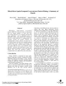
CB.2 CB.1 CB.1 WR.1 WR.2 CB.1 WR.1 CB.2 WR.2 WR.1 WR.2 CB.1 CB.2 CB.1 WR.2 WR.1 Q.1 Q.1 Q.1 Q.1 Q.1 CB.1 WR.1 CB.2 WR.2 time slot t=0 time slot t=1 time slot t=2 time slot t=3 coach sketch (a) (b) (c) (d) (e) Figure 1. An example spatio-temporal dataset to compare related approaches Table 1. Comparison of MDCOP with related work Level Group Time Interval Spatio-temporal Pattern Object Object-type Uniform Mixed Consecutive Discrete Flock Pattern [4, 11] X X X Moving Clusters [8] X X X X Mixed-drove Pattern X X X X factors such as available food and water may also affect the patterns as well. However, discovering MDCOPs is challenging for several reasons: First, the process is computationally very expensive because the interest measures are computationally complex. Second, current interest measures (i.e. the spatial prevalence measure) are not sufficient to mine such patterns, so new composite interest measures to do so must be created and formalized [7, 13]. Third, the set of candidate patterns grows exponentially with the number of object-types. Fourth, since spatio-temporal datasets are huge, computationally efficient algorithms must be developed. We create and formalize a new monotonic composite interest measure to mine interesting and non-trivial MDCOPs out of massive spatio-temporal datasets in a computationally efficient manner. Related Work: Previous studies for mining spatio-temporal co-occurrence patterns can be classified into two categories, namely, mining of uniform groups of moving objects (e.g., flock patterns [4, 11]) and mining of mixed groups of moving objects (e.g., moving clusters [8]). Our problem belongs to the latter one (Table 1). A flock pattern is a moving group of the same kind of object, such as a sheep flock or a bird flock. Gudmundsson et al. proposed algorithms for detection of the flock pattern in spatio-temporal datasets [4]. Since our problem is to mine mixed groups of objects, the proposed algorithms by Gudmundsson et al. to discover flock patterns may not be applicable to our problem. Kalnis et al. defined the problem of discovering moving clusters and proposed clustering-based methods to mine such patterns [8]. In their approach, if there is a large enough number of common objects between clusters in consecutive time slots, such clusters are called moving clusters. Moving cluster patterns can be either uniform or a mixed group of objects [8]. However if there is no overlap between the clusters in consecutive time slots, their proposed algorithms for mining moving clusters will fail to discover MDCOPs. Table 1 shows a comparison of related work and our proposed MDCOP. To illustrate the difference between our proposed MDCOP mining problem and related work (the flock pattern mining [4] and moving clusters mining [8]), we use the spatio-temporal dataset given in Figure 1, which gives an example of a spatio-temporal dataset of a typical play during an American football game. It shows the positions of two offensive wide receivers (WR.1 and WR.2), two defensive cornerbacks (CB.1 and CB.2), and a quarterback (Q.1) in four time slots. The objective is to have the two offensive wide receivers cross over each other and create a separation from the defensive cornerbacks to make it safer to receive a pass from the quarterback. Initially, the offensive wide receivers and the defensive cornerbacks are co-located at the time slot t=0 (Figure 1(a)). In time slot t=1, the two offensive wide receivers begin their run, while the defensive cornerbacks remain in their original position, possibly due to a fake handoff from the quarterback to the running back. (Figure 1(b)). In time slot t=2, the wide receivers cross over each other and try to drift further away from their respective defensive cornerbacks (Figure 1(c)). When the quarterback shows signs of throwing the football, both defensive cornerbacks run to their respective offensive wide receivers (Figure 1(d)). The overall sketch of the game tactics can be seen in Figure 1(e). The flock pattern algorithm [4] will not be able to find any pattern from the dataset given in Figure 1, since it is looking for uniform sets of moving objects. A.1 A.2 A.4 A.3 A.1 A.2 A.1 A.2 A.3 A.4 A.3 A.4 A.4 A.2 A.1 A.3 B.1 B.5 B.5 B.5 B.5 B.1 B.1 B.1 B.4 B.4 B.4 B.4 B.3 B.3 B.3 B.3 B.2 B.2 B.2 B.2 C.1 C.1 C.1 C.1 C.3 C.3 C.3 C.3 C.2 C.2 C.2 C.2 D.4 D.1 D.1 D.1 D.1 D.2 D.2 D.2 D.2 D.3 D.3 D.3 D.3 D.4 D.4 D.4 time slot t=0 time slot t=1 time slot t=2 time slot t=3 Figure 2. An input spatio-temporal dataset Spatial prevalence index values Co-occurrence Patterns time slot 0 time slot 1 time slot 2 time slot 3 Time prevalence index values A B 3/5 3/5 3/5 3/5 4/4 A C 2/4 2/4 2/4 0 3/4 B C 0 3/5 3/5 3/5 3/4 A B C 0 2/5 2/5 0 2/4 Figure 3. A set of output mixed-drove spatio-temporal co-occurrence patterns The moving clusters algorithms [8] will not be able to find any moving clusters in such an example because the wide receivers and cornerbacks are forming a cluster in time slots t=0 and t=3 but not in the intermediate time slots. Thus, there may not be any overlapping objects between clusters in consecutive time slots. In contrast, our proposed MDCOP mining approach may find MDCOP {wide_receiver, cornerback}, if the fraction of time slots where the pattern occurs over the total number of time slots is no less than a given threshold 0.5. After all, instances of MDCOP {wide_receiver, cornerback} are co-located in two time slots out of four. The instances of MDCOP {wide_receiver, cornerback} are {WR.1, CB.1} and {WR.2, CB.2} in time slot t=0, and {WR.2, CB.1} and {WR.1, CB.2} in time slot t=3.Contributions: This paper makes the following contributions:It defines mixed-drove spatio-temporal co-occurrence patterns (MDCOPs) and the MDCOP mining problem. It proposes a new monotonic composite interest measure to discover and mine MDCOPs. It proposes a novel and computationally efficient MDCOP mining algorithm (MDCOP-Miner). It shows that the proposed algorithm is correct and complete in finding mixed-drove prevalent (e.g., spatial prevalent and time prevalent) MDCOPs. It experimentally evaluates the proposed composite interest measures and MDCOP mining algorithms using real datasets. Scope: This paper focuses on the MDCOP on a typed collection of moving objects by extending interest measures for spatial co-location patterns [7, 13] given a user defined participation index threshold. The following issues are beyond the scope of this paper: (i) determining thresholds for MDCOP interest measures; (ii) similarity measures for tracking moving objects due to the focus on object-types rather than objects; (iii) indexing and query processing issues related to mining objects; (iv) discovering multisets (e.g.{A, A, B}).Outline: The rest of the paper is organized as follows. Section 2 presents basic concepts to provide a formal model of MDCOPs and the problem statement of mining MDCOPs. Section 3 presents our proposed MDCOP mining algorithm. Analysis of the algorithm is given in Section 4. Section 5 presents the experimental evaluation and Section 6 discusses conclusions and future works. 2. Basic Concepts and Problem Statement 2.1 Spatial Prevalence Measure The focus of this study is to discover mixed-drove spatio-temporal co-occurrence patterns (MDCOPs) over a spatio-temporal framework and a neighborhood relation R. First we will explain the modeling of mixed groups of object-types in space, e.g., spatial co-locations [13]. In the next sections, we will explain how we model modeling MDCOPs by extending the spatial co-location mining problem to include time information and then propose algorithms to mine these MDCOPs. Spatial co-location mining algorithms are used to discover sets of mixed object-types that are frequently located together in a spatial framework for a given set of spatial object-types, their instances, and a spatial neighbor relationship R [7, 13]. For example, in Figure 2, in time slot t=0, {A.1, C.1} is an instance of a co-location if the distance between the objects is no more than a given neighborhood distance threshold. In Figure 2, the solid lines show the distance between the objects that satisfies the neighborhood distance threshold. The participation index is used to determine the strength of the co-location pattern, that is, whether the index is greater than or equal to a threshold [7, 13]. Such a co-location is called spatial prevalent. The participation index is defined as the minimum of the participation ratios (the fraction of the number of instances on object-types forming co-location instances to the total number of instances). For example, in Figure 2, {A, B} is a co-location in time slot t=0, and its instances are {A.1, B.1}, {A.2, B.1}, {A.3, B.2}, and {A.3, B.3}. In the dataset, object-type A has 4 instances and three of them (A.1, A.2, and A.3) are contributing to the co-location {A, B}, so the participation ratio of A is 3/4. The participation ratio of B is 3/5 since 3 out of 5 instances are contributing to the co-location {A, B}. The participation index of the co-location {A, B} is 3/5, which is the minimum of the participation ratios of object-types A and B. It has been shown that the participation index is anti-monotone in size of co-locations [7, 13]. In other words, participation_index(Pparticipation_index(Pif is a subset of . In addition, [7, 13] show that the participation indexhas a spatial statistical interpretation as an upper bound on the cross-function [3]. 2.2. Modeling MDCOPs Given a set of spatio-temporal object-types and a set of their instances with a neighborhood relationship R, an MDCOP is a subset of spatio-temporal object-types whose instances are neighbors in space and time. Definition 2.1:Given a spatio-temporal pattern and a set T of time slots, such that T=[T , … , Tn-1], the time prevalence or persistence measure of the pattern is the fraction of time slots where the pattern occurs over the total number of time slots. For example, in Figure 2, the total number of time slots is 4 and pattern {A, B} occurs in all 4 time slots, so its time prevalence is 4/4. Pattern {A, C} occurs in 3 time slots, namely, time slots t=0, t=1, and t=2, and its time prevalence index is 3/4. Definition 2.2:Given a spatio-temporal dataset ST, and a spatial prevalence threshold the mixed-drove prevalence measure of a spatio-temporal pattern P is a composition of the spatial prevalence measure and the time prevalence measure as shown below. where Prob stands for probability of overall prevalence time slots and s_prev stands for spatial prevalence, e.g., the participation index, described in section 2.1. Definition 2.3:Given a spatio-temporal dataset ST and a threshold pair (time ), MDCOP P is a mixed-drove prevalent pattern, if its mixed-drove prevalence measure satisfies the following. where Prob stands for probability of overall prevalence time slots, s_prev stands for spatial prevalence, is the spatial prevalence thresholdand time is the time prevalence threshold. For example, in Figure 2, {A, B} is an MDCOP because it is spatial prevalent in time slots t=0, t=1, t=2, and t=3 since its participation indices are no less than the given threshold 0.4 in these time slots, and it is time prevalent since its time prevalence index, i.e., 1, is above the time prevalence index threshold 0.5. In contrast, pattern {B, D} is not an MDCOP. Although it is spatial prevalent in time slot t=2, it is not time prevalent since its time prevalence index is no more than the given time prevalence index threshold 0.5. 2.3. Problem statement Given: A set of Boolean spatio-temporal object-types over a common spatio-temporal framework STF. A neighbor relation R over locations. A spatial prevalence threshold, A time prevalence threshold, timeFind: is a subset of and is prevalent MDCOP as in Definition 2.3}. Objective: Minimize computation cost. Constraints: To find a correct and complete set of MDCOPs. Example: In American Football, each play (e.g., Figure 1) may represent a spatio-temporal dataset and Boolean object-types may be identified by the role of the players (e.g., wide receiver and cornerback). Each object-types are considered as Boolean because of we are interested in presence and absence at any location and time. Figure 1(a)-(d) shows the position of the Boolean object-types for four time units. The straight lines between the players show the neighboring ones. The neighbor relation R may be defined by a distance less than one meter or an average arm’s length. For example, in Figure 1(a), wide receiver WR.1 is a neighbor of cornerback CB.1. However, these players are not neighbors in Figure 1(b) since they are separated by more than a meter. In this example, {wide_receiver, cornerback} forms a candidate MDCOP,given =0.5, and time=0.5. 3. Mining MDCOPs In this section, we first discuss a naïve approachand then propose a novel MDCOP mining algorithm (MDCOP-Miner) to mine MDCOPs. Naïve approach: A naïve approach can use a spatial co-location mining algorithm for each time slot to find spatial prevalent co-locations and then can apply a post-processing step to discover mixed-drove prevalent MDCOPs by checking their time prevalence. To mine co-locations, Huang, Shekhar and Xiong proposed a join-based approach, Yoo, Shekhar and Celik proposed a partial join-based approach and a join-less approach, and Zhang et al. proposed a multi-way spatial join-based approach [2, 7, 13, 15-18]. This study will be based on the join-based spatial co-location pattern mining algorithm proposed by Huang et al., but it is also possible to use other approaches. The naive approach will generate size k+1 candidate co-locations for each time slot using spatial prevalent size k subclasses until there are no more candidate spatial co-locations. After finding all size spatial prevalent co-locations in each time slot, a post-processing step can be used to discover mixed-drove prevalent MDCOPs by pruning out time non-prevalent co-locations. Even though this approach will prune out spatial non-prevalent co-locations early, it will not prune out time non-prevalent MDCOPs before the post-processing step. This leads to unnecessary computational cost. MDCOP-Miner: In contrast, we propose an MDCOP mining algorithm (MDCOP-Miner) to discover mixed-drove prevalent MDCOPs by incorporating a time-prevalence based filtering step in each iteration of the algorithm. It will generate size k+1 candidate MDCOPs using size k mixed-drove prevalent MDCOPs. The participation index is used as a spatial prevalence interest measure to check if the pattern is spatial prevalent at a time slot [7]. The time prevalence (i.e., persistence measure in definition 2.1) is used as a time prevalence interest measure. First we give the pseudo code of the algorithm, and then we provide an execution trace of it using the spatio-temporal dataset from Figure 2. Pseudo code for MDCOP-Miner Algorithm Inputs: E: a set of spatial object-types ST: a spatio-temporal dataset object_type, object_id, x, y, time&#x-170; R : spatial neighborhood relationship TF : a time slot frame {t, ….tn-1 : a spatial prevalence threshold time: a time prevalence threshold Output: MDCOPs whose spatial prevalence indices, i.e., participation indices, are no less than , for time prevalence indices are no less than timeVariables: k: co-occurrence size t: time slots (0,….,n-1) : set of instances of size-k co-occurrences : set of candidate size k co-occurrences : set of spatial prevalent size k co-occurrences : set of time prevalent size k co-occurrences MDP : set of mixed-drove size k co-occurrences Algorithm: initialization co-occurrence size k=1, C(0)=E, MDP(0)=ST while ( not empty MDP For each time slot t in (0,….,n-1){ Ck+1(t)=gen_candidate_co-occ(C(t), MDP(t)) Tk+1(t)=gen_co-occur_instance(Ck+1(t), T(t), R) SPk+1(t)=find_spatial-prevalent_co-occ(Tk+1(t),Ck+1(t) } TPk+1=find_time_prevalence_index (SPk+1 MDPk+1=find_time-prevalent_co-occur (TPk+1timereturn union (MDP, ….. MDPk+1 Algorithm 1. MDCOP-Miner algorithm Algorithm 1 gives the pseudo code of the MDCOP-Miner algorithm. The inputs are a set of spatial object-types E, a spatio-temporal dataset ST, a spatial neighborhood relationship R, and thresholds of interest measures, i.e. spatial prevalence and time prevalence and the output is a set of mixed-drove prevalent MDCOPs. (a) (b) Figure 4. Execution trace of the MDCOP-Miner algorithm In the algorithm, steps 1 and 2 include initialization of the parameters, steps 3 through 12 give an iterative process to mine MDCOPs, and step 13 gives a union of the results of the iterative steps. Steps 3 through 12 continue until there is no candidate MDCOPs to be generated (mined). The functions of the algorithm are explained below. Generation of candidate co-occurrence patterns (step 5): This function uses an apriori-based approach to generate size k+1 candidate co-locations Ck+1 for each time slot, using all mixed-drove prevalent size k mixed-drove co-occurrence patterns MDP [1].Generating spatial co-occurrence instances (step 6):The instances of candidate Ck+1 are generated by joining neighbor instances of mixed-drove prevalent size k MDCOPs for each time slot. This is similar to the instance generation step of the co-location miner algorithm [7]. Finding spatial prevalent co-occurrence patterns (step 7): All spatial prevalent size k+1 patterns SPk+1 are found by pruning the patterns whose spatial prevalence indices, i.e., participation indices, are less than a given threshold for each time slot. Computation of the participation indices follows the same algorithmic ideas as those in the co-location mining algorithm [7]. In steps 5 through 7, the algorithm finds size k+1 spatial prevalent co-locations for each time slot.Forming a time prevalence table (step 9): In step 9, the time prevalence indices of the mined spatial prevalent patterns are calculated. The time prevalence index of a spatial prevalent co-location is the fraction of the number of time slots where the pattern occurs over the total number of the time slots.Finding mixed-drove co-occurrence patterns (step This step discovers MDCOPs by checking the time prevalence indices of the spatial prevalent co-locations if they are no less than a given time prevalence threshold time . The patterns whose time prevalence indices do not satisfy the given threshold are pruned at this stage. The remaining patterns will be mixed-drove prevalent MDCOPs and will be used to generate candidate supersets of the MDCOPs in step 5. The algorithm will run iteratively until there are no more candidate MDCOPs to be generated. The algorithm outputs the union of all size mixed-drove prevalent MDCOPs. An Execution Trace: The execution trace of the algorithm is given in Figure 4 using the spatio-temporal dataset given in Figure 2. This dataset contains four object-types A, B, C, and D and their instances in four time slots. A has 4 instances, B has 5 instances, C has 3 instances, and D has 4 instances. The instances of each object-type have a unique identifier, such as A.1. Some of the patterns of these object-types form an MDCOP. To discover MDCOPs we propose a monotonic composite interest measure (the mixed-drove prevalence measure) which is a composition of the spatial prevalence and time prevalence measures. The spatial prevalence measure, (participation index) shows the strength of the spatial co-location when the index is greater than or equal to a given threshold [7, 13].The time prevalence measure (time prevalence index) shows the frequency of the pattern over time. In Figure 4(a), in step 1, candidate spatial co-location pairs of the object-types and their instances are generated for each time slot. The spatial co-locations whose participation indices are less than a given threshold are then pruned. A spatial non-prevalent co-location {A, D} is pruned in time slot t=0, {C, D} is pruned in time slots t=2 and t=3, and {B, D} is pruned in time slots t=3 because their participation indices are less than the given threshold 0.4. A time prevalence table of pairs of spatial prevalent co-locations is then formed by entering a 1 if the participation index of the corresponding pattern satisfies a given participation index threshold. Time-prevalence indices are then found. For example, in the time prevalence table (step 2 in Figure 4(b)), spatial prevalent pattern {A, B} is persistent for all time slots and its time prevalence index is 4/4, and spatial prevalent pattern {A, C} is persistent in time slots t=0, t=1, and t=2 and its time prevalence index is 3/4, etc. The MDCOPs whose time prevalence indices are no less than a given threshold are selected for generating superset candidate MDCOPs. Spatial prevalent patterns {A, B}, {A, C}, and {B, C} are selected as mixed-drove prevalent MDCOPs since they are also time prevalent (their time prevalence indices satisfy the given time prevalence index threshold 0.5). In contrast, spatial prevalent patterns {A, D}, {B, D}, and {C, D} are pruned since they are time non-prevalent. Using MDCOPs {A,B}, {A, C}, and {B, C}, the next candidate MDCOP {A, B, C} is generated. The next step is to generate instances of candidate MDCOP {A, B, C} in time slots where its subsets exist and to check its participation indices in these time slots. Since all subsets of MDCOP {A, B, C} are mixed-drove prevalent MDCOPs and exist in time slots t=1 and t=2, there is no need to generate instances of them for time slots t=0 and t=3. In step 3 (Figure 4(b)), the instances of candidate MDCOP {A,B,C} are generated and participation indices are found which are 2/5 for time slots t=1 and t=2. In step 4 (Figure 4(b)), the time prevalence table is formed for pattern {A, B, C} and its time prevalence index is checked to see if it satisfies the time prevalence threshold. Candidate MDCOP {A, B, C} is an MDCOP since its time prevalence index 0.5 is equal to the time prevalence threshold 0.5. Since there are not enough subsets to generate the next superset patterns, the algorithm stops at this stage and outputs the MDCOPs union of all size mixed-drove prevalent MDCOPs, i.e., {A, B}, {A, C}, {B, C}, and {A, B, C}. 4. Analysis of the MDCOP-Miner This section gives the analysis of the mixed-drove prevalence index measure, and correctness and completeness derviations for the MDCOP-Miner. 4.1. The Mixed-Drove Prevalence Index Measure is Monotonic Lemma 4.1:A chosen spatial prevalence measure, e.g., participation index, is monotonically non-increasing in the size of the MDCOPs at each time slot [7, 13]. Lemma 4.2:A mixed-drove prevalence index measure is monotonically non-increasing with the size of MDCOP over space and time. In other words, if MDCOP P is a subset of MDCOP P , andwhere Prob stands for probability of overall prevalence time units, s_prev stands for spatial prevalence, is spatial prevalence thresholdand time slot. Proof: The basic proof sketch follows. Let Lemma 4.1 implies that for all , since is a subset of , Thus, where is time prevalence threshold. 4.2. Correctness and Completeness Theorem 4.1:The MDCOP-Miner is complete. Proof: The MDCOP-Miner is complete if it finds all prevalent mixed-drove prevalent MDCOPs that satisfy a given participation index threshold and time prevalence threshold. We can show this by proving that none of the functions of the algorithm miss any patterns, i.e., filter out a prevalent MDCOP. The gen_candidate_co-occur function does not miss any patterns given the anti-monotone nature of the MDCOP interest measure. The input of this function is mixed-drove prevalent size k MDCOPs and the output is candidate size k+1 MDCOPs. If ={f,…,f} and c={f,…fk-1k+1} are size k mixed-drove prevalent MDCOPs, candidate size k+1 pattern k+1={f,… fk-1k+1} will be produced by joining mixed-drove prevalent size k MDCOPs. The gen_co-occur_instanance function does not miss any patterns. This function generates instances of candidate size k+1 MDCOPs by joining instances of mixed-drove prevalent size k MDCOPs if they are in the neighborhood distance and forming a clique. The find_spatial-prevalent_co-oc function does not miss any patterns. It finds spatial prevalent patterns whose participation indices satisfy a given threshold. The find_time_prevalence_index function does not miss any patterns. This function calculates time prevalence indices of the patterns found in steps 4 through 8 and does not do any pruning. The find_time-prevalent_co-occur function does not miss any MDCOP. The function finds all the mixed-drove prevalent MDCOPs whose time prevalence indices are no less than a given threshold. Theorem 4.2:The MDCOP-Miner is correct. In other words, if a MDCOP pattern P is returned by MDCOP-Miner algorithm then P is a prevalent MDCOP.Proof: The proof is easy to establish due to the pruning steps of “find_spatial_prevalent_co-occur”, and find_time_prevalent_co-occur” which weed out candidates not meeting the given thresholds. Theorem 4.3: The total cost of MDCOP-Miner algorithm is no more than the total cost of naïve approach. Proof: The basic proof sketch follows. MDCOP-Miner prunes out spatial prevalent but time non-prevalent patterns early and generates no more candidates than the Naïve approach. The cost of time pruning is negligible relative to the spatial pruning. 5. Experimental Evaluation In this section, we present our experimental evaluations of several design decisions and workload parameters of our MDCOP-Miner algorithm. We used a real-world training dataset. We evaluated the behavior of the MDCOP-Miner and naive approach by changing the number of time slots, number of object-types, and the spatial prevalence and time prevalence index thresholds. Figure 5 shows the experimental setup to evaluate the impact of design decisions of the performance of both algorithms. Experiments were conducted on an Intel Centrino PIV 1.6 GHz computer with 512 MB of RAM. MDCOP Mining Algorithms Real Dataset Candidate Algorithms(Naïve, MDCOP-Miner) Analysis Measurements Number of Time Slots Number of features Time Prevalence Threshold Spatial Prevalence ThresholdFigure 5. Experimental setup and design The dataset contains the location and time information of moving objects. It includes 15 time snapshots and 22 distinct vehicle types and their instances. The minimum instance number is 2, the maximum instance number is 78, and the average number of instances is 19. Figure 6 shows an instance of an MDCOP. Object_1 and object_2 are coming together, moving from top right to bottom left. Such a pattern may be of interest if it indicates an imminent offensive maneuver by object_1 under cover from object_2. Figure 6. One instance of an MDCOP 5.1 Effect of Number of Time slots In the first experiment, we evaluated the effect of number of time slots on the execution time of both algorithms. The participation index, time prevalence index, and distance were set at 0.15, 0.5, and 100m respectively. The MDCOP-Miner requires less execution time than the naive approach, since it prunes out mixed-drove non-prevalent MDCOPs early (Figure 7). It can also be seen that, as the number of time slots increases, the ratio of the increase in execution time is smaller for MDCOP-Miner than the naïve approach. Figure 7. Effect of number of time slots 5.2 Effect of Number of Object-types In the second experiment, we evaluated the effect of number of object-types on the execution time of both algorithms. The participation index, time prevalence index, number of time slots and distance were set at 0.15, 0.5, 15, and 100m respectively. The MDCOP-Miner outperforms the naive approach as the number of object-types increases (Figure 8). It is observed that the increase ratio of the execution time of the naive approach is bigger than the MDCOP-Miner as the number of object-types increases. It should also be noted that the distributions of the object-types affect the computation cost of both algorithms. The cost of both algorithms increases dramatically between 16 and 20 since the newly added 4 object-types are highly likely to have neighbor relations with nearby object-types. In contrast, between 20 and 22, the cost does not increase too much since the newly added object-types are less likely to have neighbor relations with nearby object-types. Figure 8. Effect of number of object-types 5.3 Effect of the Time Prevalence Index Threshold In the third experiment, we evaluated the effect of the time prevalence index threshold on the execution times of both algorithms. The fixed parameters were participation index, number of time slots, and distance, and their values were 0.15, 15, and 100m respectively. For the naïve approach, the effective cost in execution time to generate spatial prevalent co-locations will be constant since it generates the same number of spatial prevalent patterns as the time prevalence index increases. In that case, the cost of the post-processing step will reflect the trend of the naive approach. Experimental results show that the MDCOP-Miner is more computationally efficient than the naive approach because of the early pruning strategy (Figure 9). It is also observed that the naive approach is computationally more expensive as the time prevalence index threshold decreases because of the increase in the number of MDCOPs to be discovered. Figure 9. Effect of the time prevalence index threshold 5.4 Effect of the Spatial Prevalence Index Threshold In the fourth experiment, we evaluated the effect of the spatial prevalence index threshold on the execution times of both algorithms. The fixed parameters are time prevalence index, number of time slots, and distance, with values of 0.5, 15, and 100m respectively. The MDCOP-Miner outperforms the naive approach as the spatial prevalence index threshold increases (Figure 10). The cost of the naive approach will be higher than the MDCOP-Miner for low values of the spatial prevalence index threshold. Figure 10. Effect of spatial prevalence index threshold It is also observed in all the experiments that the memory usage of the MDCOP-Miner is no more than for the naïve approach (Theorem 4.3). 6. Conclusions and Future Work We defined mixed-drove spatio-temporal co-occurrence patterns (MDCOPs) and the MDCOP mining problem and proposed a new monotonic composite interest measure (the mixed-drove prevalence measure), which is the composition of the spatial prevalence and time prevalence measures. We also presented a novel and computationally efficient algorithm (the MDCOP-Miner) for mining these patterns. We compared our algorithm with a naive approach, which runs the spatial co-location mining algorithm at each time slot and then discovers MDCOPs using a post-processing step. We proved that the proposed algorithms are correct and complete in finding mixed-drove prevalent (e.g., spatial-prevalent and time prevalent) MDCOPs. Our experimental results using a real dataset provide further evidence of the viability of our approach. In future work, we would like to evaluate effect of objects (instances) of object-types on the proposed algorithms andto explore the relationship between the proposed MDCOP interest measures and the spatio-temporal statistical measures of interaction [2]. Another problem of interest is the characterization of the probability distribution of the proposed interest measure to help in making the choice of thresholds in the proposed measures. We plan to explore other potential interest measures for MDCOPs by evaluating similarity measures for tracks of moving objects. We plan to investigate new monotonic composite interest measures and develop new computationally efficient algorithms for mining MDCOPs. In the literature, there also other studies focused on defining spatio-temporal patterns and algorithm [4, 6, 8, 10, 12, 14]. Laube and Imfeld defined several spatio-temporal patterns, such as, leadership, convergence [11]. Query processing algorithms have been proposed to extract such patterns [11]. We plan to extend our algorithm to mine these patterns. 7. Acknowledgments The authors would like to thank James Kang and Kim Koffolt for their comments. 8. References [1] R. Agarwal and R. Srikant, Fast algorithms for Mining Association Rules, VLDB'94, 1994. [2] S. Banerjee, B. P. Carlin, and A. E. Gelfrand, Hierarchical Modeling and Analysis for Spatial Data, CRC Press, ISBN 158488410X, 2003. [3] N. A. C. Cressie, Statistics for Spatial Data, Wiley and Sons, ISBN 0471843369, 1991. [4] J. Gudmundsson, M. v. Kreveld, and B. Speckmann, Efficient Detection of Motion Patterns in Spatio-Temporal Data Sets, ACM-GIS,250-257, 2004. [5] R. Guting and M. Schneider, Moving Object DatabasesMorgan Kaufmans, 2005. [6] M. Hadjieleftheriou, G. Kollios, P. Bakalov, and V. J. Tsotras, Complex Spatio-Temporal Pattern Queries, VLDB'05,877-888, 2005. [7] Y. Huang, S. Shekhar, and H. Xiong, Discovering Co-location Patterns from Spatial Datasets: A General Approach, IEEE Trans. on Knowledge and Data Eng. (TKDE), vol. 16(12), pp. 1472-1485, 2004. [8] P. Kalnis, N. Mamoulis, and S. Bakiras, On Discovering Moving Clusters in Spatio-temporal Data, 9th Int'l Symp. on Spatial and Temporal Databases (SSTD), Angra dos Reis, Brazil, 2005. [9] M. Koubarakis, T. Sellis, A. Frank, S. Grumbach, R. Guting, C. Jensen, N. Lorentzos, H. J. Schek, and M. Scholl, Spatio-Temporal Databases: The Chorochronos Approach, LNCS , vol. 9, Springer Verlag, 2003. [10] P. Laube and S. Imfeld, Analyzing relative motion within groups of trackable moving point objects, in In GIScience, number 2478 in Lecture notes in Computer Science. Berlin: Springer, pp. 132-144, 2002. [11] P. Laube, M. v. Kreveld, and S. Imfeld, Finding REMO - detecting relative motion patterns in geospatial lifelines, 11th Int'l Symp. on Spatial Data Handling,201-214, 2004. [12] C. d. Mouza and P. Rigaux, Mobility Patterns, GeoInformaticavol. 9(4), pp. 297-319, 2005. [13] S. Shekhar, Y. Huang, and H. Xiong, Discovering Spatial Co-location Patterns: A Summary of Results, 7th Int'l Symp. on Spatial and Temporal Databases (SSTD), L.A., CA, 2001. [14] H. Yang, S. Parthasarathy, and S. Mehta, A Generalized Framework For Mining Spatio-temporal Patterns in Scientific Data, ACM SIGKDD Int'l Conf. on Knowledge Discovery and Data Mining (SIGKDD),716-721, 2005. [15] J. S. Yoo and S. Shekhar, A Joinless Approach for Mining Spatial Colocation Patterns, IEEE Trans. on Knowledge and Data Eng. (TKDE), vol. 18(10), pp., 2006. [16] J. S. Yoo and S. Shekhar, A Partial Join Approach for Mining Co-location Patterns, ACM-GIS'05, Washington D.C., USA, 2005. [17] J. S. Yoo, S. Shekhar, and M. Celik, A Join-less Approach for Co-location Pattern Mining: A Summary of Results, IEEE Int'l Conf. on Data Mining, Houston, USA, 2005. [18] X. Zhang, N. Mamoulis, D. W. L. Cheung, and Y. Shou, Fast Mining of Spatial Collocations, 10th ACM SIGKDD Int'l Conf. on Knowledge Discovery and Data Mining,384-393, Seatle, WA, 2004.