Acoustic Upside-down Levitator With A Solid Sample - PowerPoint Presentation

Slide1

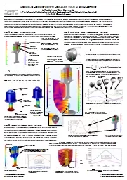
Acoustic Upside-down Levitator With A Solid SampleLothar Holitzner1, Ernst Günter Lierke21. Paul Scherrer Institut, Laboratory for Scientific Developments and Novel Materials, Villigen, Switzerland; 2. tec5 AG, Oberursel, Germany.

Introduction:Acoustic levitators are used to levitate small samples (ca. 0.01 - 6 mm) at a stable position in a gaseous or liquid environment. Acoustic levitators were first developed und used for experiments in space (1970s, by NASA / ESA), the application later became terrestrial (1990s). Meanwhile acoustic levitators are widespread. With the help of COMSOL Multiphysics® , we present a practical model, to show basic properties and interactions and some additional phenomena und aspects in a stepwise approach to the realistic world of acoustic levitators. In this acoustic levitator model the millimetre-sized spherical sample is located (in air environment) below the piezoelectric transducer (mechanical coupled resonator), which radiates the inaudible sound of 22 kHz downwards against the reflector. The transducer is based on a sophisticated 20 kHz model, designed by E.-G. Lierke. That version was also used at the Battelle Institute (Frankfurt/Main, Germany) [1]. The current available model contributes to understand details of acoustic levitation and helps to improve acoustic levitators for future applications.

[2] Alon Grinenko, How to Compute the Acoustic Radiation

Force, COMSOL BLOG, January 29, 2015 [3] Mads Herring Jensen, COMSOL Support Case 3000332, 2018

Figure 9.

Snapshot of the axial stress in the transducer. (deform. scale factor = 3000)

Study 4: Transducer motion (Time Dependent) This study explores the transduceroscillation at the resonance frequency(22 kHz) in timewise resolved motionsequence.

Figure 8.

Transducer displacement field, Z-component, resp. piezo voltage during swing up.

Figure 7.

Input

: Electrical power, calculated from piezo current and voltage

. Output: Acoustically radiated power, calculated at the sonotrode face boundaries

Study

3

: Frequency scan (Frequency Domain, prestressed) A frequency domain study (Harmonic Perturbation) vibrates the prestressed piezoelectric transducer to harmonic oscillations (with use of the AC/DC Module). The frequency scan over the resonance range also shows the internal mechanical (Rayleigh) Damping in the transducer material with the shape of the amplitude resonance curve (reasonable damping values taken from e.g. annealed high-grade titanium alloy). The Acoustics Module was used, to calculate the Acoustic-Solid Interaction between transducer, acoustic levitation field, reflector and solid sample. The oscillating transducer radiates its maximum power into the gas domain, when the distance between sonotrode face and (spherical curved) reflector is tuned to resonance, namely at max. acoustic impedance.

Fig. 6 shows an optimized intense sound field with 5 stationary pressure nodes in the acoustic standing wave. A sample sphere Ø4mm is placed in the 3rd pressure node. Fig. 7 indicates the frequency-dependent power transfer on the way from the piezo electrodes into the levitation sound field. (Note: Fig. 4 to Fig. 7 with Upiezo = 7 Vrms )

Figure 6.

Sound pressure level in the gas domain beween transducer and reflector

reflector

sound field

3rd pressure

node

Figure 5.

Displacement amplitude, z-component.

Figure 4.

Displacement amplitude at

22000 Hz

Ti6Al4V (3.7165)

Rayleigh damping

with material quality factor Q = 1500

- resulting mass damping parameter α = 45.936 [1/s]- resulting stiffness damping parameter β = 2.409e-9 [s]

stainless steel (1.4435)

sonotrode

face

AC voltage

(Harmonic

Pertubation)

[1] L. Holitzner, Verbesserung der Funktions-Charakteristik eines elektrostatisch akustischen Hybridlevitators, FH Wiesbaden, Battelle Institut, Frankfurt/M., 1992

Study

6

: Sample position balance (Frequency Domain, prestressed)

The mesh of the gas domain, which locally surrounds the solid sample, is based on a

Moving Mesh

and enables the sample domain to change its position. The 1

st

study step (Stationary) calculates the final vertical sample position with a simple force balance equation, defined in

Global ODEs and DAEs (ge) and moves the sample by a Prescribed Displacement. The mesh in the sample proximity deforms accordingly. Then, the 2nd study step (Frequency Domain Perturbation) recalculates the pressure acoustics field in the new geometric situation. This confirms the force equilibrium between sample weight and vertical acoustic radiation forces on the sample surface.

Figure 11. Stable levitated sample in force equilibrium at vertical balance position below the 3rd pressure node

Figure 10

.

Vertical force Faco.z from acoustic radiation pressure at different vertical sample positions. Faco.z = Faco.bottom + Faco.top

pressure node position

The levitation force progression can be investigated with a

Parametric Sweep

of the vertical sample position over the pressure node region. This force progression is used as an input to study 6.

Study

5

: Sample position scan

(

Freq.

Domain)

The acoustic radiation pressure from the intense sound field acts on the sample surface and creates forces, which try to push the sample into the pressure node.

The

vertical force

F

aco.z

on the sample

surface is calculated (see [2]) with field variables from the interface Pressure Acoustics (acpr). After [3] the deformation degree of freedom of the structure is used to get the velocity at the sample surface Ssample .

Study

2

: Transducer geometry (Eigenfrequency, prestr.) In the 2nd development step, an eigenfrequency study inspects the undamped, axial natural oscillation of the prestressed piezoelectric transducer. By adjusting the transducer geometry, the resonance frequency was tuned to 22 kHz and the velocity node placed into the level of the fixing flange. This Eigenfrequency study also helps, to exclude undesired tilt and pendulum oscillations of the transducer.

Figure 2.

Total displacement (amplitude) at transducer Eigenfrequency 22002 Hz (deformation scale factor = 500)

fixing flange

(velocity node)

sonotrode

driver

(velocity antinode)

(velocity antinode)

Figure 3.

Undesired oscillation at

19963 Hz

(deformation scale

factor = 130)

Study

1

: Piezo preload (Stationary, prestressed)

In the 1st development step of the FEM model, only the transducer was set up and the Structural Mechanics Module was used for a stationary study. In this transducer assembling

step, the piezo rings of the transducer are axially preloaded by the central clamping screw (Bolt Pre-Tension). With open piezo electrode ports, the resulting piezo voltage indicates the mechanical preload in practice (Piezoelectric Effect).

region with resulting

compressive stress

bolt under

pre-tension

resulting

piezo voltage

(Floating Potential)

Figure 1.

Piezo voltage and axial stress after prestressing the central bolt.