Gate Set Tomography Kenneth Rudinger - PowerPoint Presentation

Slide1

Gate Set Tomography

Kenneth Rudinger

Slide2

Outline

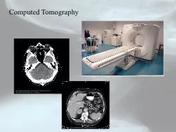
Motivation for quantum tomography

Framework for self-consistent, calibration-free tomography:

Gate set tomographyAchieving Heisenberg accuracy scaling with gate set tomographyUsing gate set tomography to build a better trapped ion qubit at Sandia National Laboratories

3

Slide3

Towards true QIP

4

Slide4

Towards true QIP

5

Slide5

Towards true QIP

6

Slide6

Towards true QIP

7

Slide7

8

Goal of tomography:

Make

ε

ij

as small as possible as cheaply as possible.

Slide8

The problem with tomography

Critical problem: relies on

precalibrated

reference frames that

don’t

really exist in hardware!

Goal: Calibration-free tomography.

9

Slide9

“Black box picture” of quantum information processor

10

Slide10

“Black box picture” of quantum information processor

prepare

do experiments

measure

outcome

11

Slide11

“Black box picture” of quantum information processor

prepare

do experiments

measure

outcome

12

Slide12

“Black box picture” of quantum information processor

prepare

do experiments

measure

outcome

Markovian

model:

13

Slide13

Perform collection of experiments.

Compute:

Gate Set Tomography Framework

Many choices for gate strings, estimator

F

.

Slide14

Gate Set Tomography

Simplest algorithm: Linear Inversion (LGST)

“Process

tomographywithout calibration”.

15

Slide15

Gate Set Tomography

Simplest algorithm: Linear Inversion (LGST)

“Process

tomographywithout calibration”.

16

Slide16

Linear gate set tomography

Use unknown gates as uncalibrated “fiducials”.

Run “process tomography” on each gate,

and on empty gate string.

17

Linear algebra

 gate set.

arXiv:1310.4492

Slide17

How does LGST perform?

18

“RMS Frobenius distance”:

Slide18

19

LGST on simulated data

Slide19

LGST review

N increases:

ε

0 No self-calibration problem

Experimentally demonstrated

i

ε

decreases slowly. (N

-0.5

)

Can we do better?

20

Slide20

21

Want to be sensitive to small errors.

Slide21

Push :

22

Need

Ο(θ

-2

)

measurements to distinguish from

I.

Slide22

Push L times:

23

Can amplify coherent errors!

Slide23

24

Slide24

25

Can each experiment just be a different gate repeated many times?

e.g. G

x

2

, G

x

4

,..., G

y

2

, G

y

4

...

Not sufficient. Need to amplify other errors as well.

e.g. Tilt error

Also want sequences like

G

x

G

y,

(G

x

G

y

)

2

, (G

x

G

y

)

4

...

Slide25

26

Call these short sequences

germs.

Germs chosen to amplify errors. (E.g. tilt, over-rotation, dephasing.)

Do LGST on successively longer “powers”.

We call this

extended linear gate set tomography (

eLGST)

.

Can instead minimize

χ

2

:

Least Squares gate set tomography (LSGST)

.

Long-sequence GST

Slide26

Minimize total

χ

2

at each step.

Does estimate fit data?

27

Slide27

Algorithm summary

Start with experimental gate set, eg. {

Gi

, Gx

,

Gy

}

From knowledge of target gate set,

determine set of germs e.g.

{

Gx

,

Gy

,

Gi

,

GxGy

,

GxGyGi

,

GxGiGy

,

GxGiGi

,

GyGiGi

,

GxGxGiGy

,

GxGyGyGi, GxGxGyGxGyGy}

For varying maximum sequence length (L=1,2,…,512), perform “process tomography” experiments on each “extended germ”

Using

least-squares

, iteratively find gate set estimates that minimize

χ

2

.

Compare to target gate set.

28

Slide28

How do we measure success?

Can we find accurate estimate cheaply? (Can we beat N

-0.5

?)

Can we diagnose

and improve

experimental qubits?

29

Slide29

How do we measure success?

Can we find accurate estimate cheaply? (Can we beat N

-0.5

?)

Can we diagnose

and improve

experimental qubits?

30

Slide30

How do we measure success?

Can we find accurate estimate cheaply? (Can we beat N

-0.5

?)

Can we diagnose

and improve

experimental qubits?

31

Slide31

32

Slide32

33

Slide33

34

Slide34

35

Slide35

GST on real systems –

c

2

analysisEach box = 1 gate string

Color =

c

2

for that string

Blue

boxes = fits well

Red

boxes = fits poorly

Line-fitting analogy:

36

(

GxGy

)

4

d

ata points

b

est fit line

Length of gate string

Germ (to repeat)

Slide36

37

April 2014:

Slide37

38

4/14:

BB1 pulses

May, 2014

Slide38

39

4/14:

5/14

Drift control

December,

2014

BB1

pulses

Slide39

40

4/14:

5/14

Drift control

12/14

BB1

pulses

Improved Gi compensation

February,

2015

Slide40

How good are these gates?

41

GST

High-fidelity gates

Markovian behavior

Enabled by GST

Slide41

Conclusions

GST yields reliable, highly accurate estimates far more cheaply than standard tomography.

GST can diagnose the presence of non-Markovian noise.

GST is being used in the construction of reliable, high-fidelity experimental gates.

42

Slide42

Future directions

Multi-qubit systems

Randomized benchmarking predictions

Non-Markovian analysisDrift control.

More experimental implenetation

Contact me!

kmrudin@sandia.gov

Thank you!

Gnome image courtesy of

http://

sweetclipart.com

/friendly-garden-gnome-1464

43

Slide43

Bonus slides!

44

Slide44

The gauge

GST predictions are

gauge-invariant

:Given a target gate set, can

gauge-optimize

estimated gate set, yielding an “easy-to-read” interpretation.

45

Slide45

New end user infrastructure

Automated report generation

Explains GST to end user

Provides best GST estimate, along with relevant scoring parametersFidelity, trace distance, rotation axes and anglesc2 plots

Diagnostic “whac-a-mole” plots

Website interface for end user to generate own reports.

https://prod.sandia.gov/gst/index.html

Generation takes ~1 minute, depending on data set.

46

Slide46

Experimental error quantification

Can’t use ||.||

F

error for experimental data (don’t know G_true)c2 gives goodness-of-fit; what about error bars on individual gate set parameters?

Tackled experimental error bars in three ways:

Hessian of

c

2

function (in progress)

Parametric bootstrapping

Non-parametric bootstrapping

47

Slide47

Bootstrapping error bars

Non-parametric bootstrapping:

Randomly take subsamples of experimental dataset many times to generate new datasets

Run GST on each new dataset; generate ensemble of gate sets.Compute spread (or other statistics) of new ensemble of gate sets.

48

Slide48

Bootstrapping error bars

Parametric bootstrapping:

Compute GST estimate of experimental dataset.

Use GST estimate to generate many new datasets.Run GST on each new dataset; generate ensemble of gate sets.Compute spread (or other statistics) of new ensemble of gate sets.

49

Slide49

Bootstrapping results

50

Slide50

51

Bootstrapping error bars

Slide51

52

Bootstrapping error bars

Parametric marginally “better” than non-parametric.

Error bars about 10

-5

to 10

-4

in size for gate elements (larger for SPAM parameters)

This information can also be included in automated GST reports.

Slide52

In a method similar to bootstrapping, we can simulate RB experiments given GST data. (Below is SNL ion data.)

Experimental decay rate: 4.9

.

10

-5

GST-predicted decay rate: 4.0

.

10

-5

Can we obviate the need for RB experiments?

53

GST vs. RB

Slide53

What about germ selection?

How do we choose germs which amplify

all

(non-SPAM) parameters?

54

Slide54

What about germ selection?

55

If {

s

i

}

is incomplete,

Q

diverges. Then ||.||

F

behaves poorly.

If

Q

does not diverge, then ||.||

F

behaves well (L

-1

scaling).

We’ve written both integer and convex programs to find “good” germ sets.

This has allowed us to find relatively small germ sets for large gate sets (e.g. 40 germs for gate set with 9 gates).

Slide55

56

What about germ selection?

We

thought that minimizing Q (or finite-L

variants thereof) should correlate to minimizing ||.||

F

.

Found the error in derivation;

need to work out correction.

Slide56

Current 1-qubit GST analysis requires ~10

3

different gate sequences to perform.

Without any changes to GST paradigm, 2-qubit GST would require ~105 unique gate sequences.(162

fiducials, ~80 germs, 10 length sequences)

…This is a lot. Can we somehow reduce number of sequences?

Lots of redundancy.

57

Future work: resource reduction

Slide57

Future work: resource reduction

58

Reduce number L’s used?

Here we see a 3-fold reduction in number of 1-qubit experiments at a cost of only a factor of 3 in accuracy.

Can we similarly throw out various sequences (L values, fiducials, germs) for 2-qubit GST to get dramatic reduction in sequence requirement?

Slide58

Can we use germ selection techniques to pick out various long gate sequences that always amplify errors?

“Derandomized benchmarking?”

Can we use model selection techniques with GST to diagnose quantum devices of unknown a priori dimension?

Thanks!59Additional future work