An examination of the chaotic magnetic field near the - PowerPoint Presentation

Slide1

An

examination of the chaotic magnetic field near the

separatrix

of magnetically confined

plasmas

S.R.Hudson

(PPPL) & Y. Suzuki (NIFS

)Slide2

T

he most important theoretical/numerical calculation

in the study of magnetically confined plasmas

is to determine the magnetic field.

MHD equilibrium codes (such as HINT-2) determine the structure of the magnetic field, allowing for islands and chaotic

fieldlines

, in

stellarators

, perturbed tokamaks, . .

It is always useful, and often essential, to know the chaotic structure of the

fieldlines

.

The efficiency, reliability and accuracy of such codes depend on accurate, robust, fast numerical routines.

Constructing efficient subroutines requires tedious, careful work

!Slide3

So, given the vector field,

B(x)

, what are the properties of the

integral-curves

≡

fieldlines

?Slide4

The simplest diagnostic:

Poincaré

plot:

from given (R,Z), follow along

B

a “distance” of

Δφ

=2

πSlide5

The simplest diagnostic:

Poincaré

plot:

from given (R,Z), follow along

B

a “distance” of

Δφ

=2

π

m

agnetic axis

“X” pointSlide6

The magnetic axis and X-point are fixed points of the

Poincaré

mapping; which may be found, for example,

using

fieldline

tracing + Newton iterations.Slide7

Example: locating the magnetic axis using

fieldline

tracing method + Newton iterations

.

(0)

(1)

(2)Slide8

“Global integration” is much faster:

t

he action integral is a functional of a curve in phase space.Slide9

The tangent mapping determines the behavior of nearby

fieldlines

.

Chaos: nearby

fieldlines

diverge exponentially. Slide10

The

Lyapunov

exponent can distinguish chaotic trajectories,

but it is computationally costly.

b

lack line = linear separationSlide11

“Global integration” can robustly find the

action minimizing curve = X-point

These constraints must be invertible.Slide12

From “arbitrary” initial guess,

e.g. from close to the O-point,

t

he gradient-flow method converges on X-point,

e

ven if the initial guess is outside the

separatrix

.

“Global integration” can robustly find the

action minimizing curve = X-pointSlide13

The magnetic axis is a “stable” fixed point (usually),

a

nd the X-point is “unstable”.

Consider the eigenvalues of tangent mapping: Slide14

The

stable

/

unstable

direction forwards in

φ

is the

unstable

/

stable

direction backwards in

φ

.

unstable

stable

separatrixSlide15

For perturbed magnetic fields, the

separatrix

splits.

A “partial”

separatrix

can be constructed.

ASDEX-USlide16

For JT60-SA, the partial

separatrix

is strongly influenced by an “almost” double-null.

JT60-SASlide17

free-streaming along field line

particle “knocked”

onto nearby field line

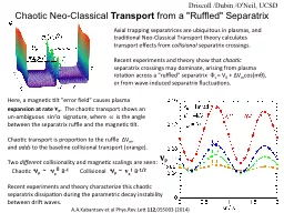
Consider heat transport:

r

apid transport along the magnetic field,

slow

transport across the magnetic field.Slide18

Anisotropic heat transport + unstable manifold = ?

What is the temperature in the “chaotic edge” ?Slide19

Anisotropic heat transport + unstable manifold = ?

What is the temperature in the “chaotic edge” ?Slide20

OCULUS: the eye into chaos

OCULUS

©

: a user-friendly,

theoretically-sophisticated

, imaginatively-named, library of subroutines for analyzing the structure of non-

integrable

(chaotic) magnetic fields

* freely available online at

http://w3.pppl.gov/~

shudson/Oculus/oculus.pdf

* 9 subroutines are presently available

This library is integrated into HINT-2, M3D-C

1,

SPEC, and NIMROD (under construction), . . .

Our long-term goal is for all high-performance codes to use shared, co-developed, freely-available, numerical libraries.

A

community-based

approach to large-scale computing.

Many codes ask the same questions, i.e. need the same subroutines.

Where is the last, closed, flux surface? Where is the unstable manifold?

W

here are the magnetic islands, and how big are they? Where is the magnetic axis? How “chaotic” is the magnetic field?Slide21
Slide22

So far, have used cylindrical coordinates (R,

φ

,Z).

Is it better to use toroidal coordinates, (

ψ

,

θ

,

φ

) ?

Fig. 6. Hudson & Suzuki,

[

PoP

, 21:102505, 2014 ]

ψ

θSlide23

Question

:

can a

toy Hamiltonian be “fit” to the partial

separatrix

to provide suitable, “background” toroidal coordinates

?

“Toy”

ASDEX-USlide24

Question

:

can a

toy Hamiltonian be “fit” to the partial

separatrix

to provide suitable, “background” toroidal coordinates

?Slide25

Question

:

can a

toy Hamiltonian be “fit” to the partial

separatrix

to provide suitable, “background” toroidal coordinates

?Slide26

Question

:

can a

toy Hamiltonian be “fit” to the partial

separatrix

to provide suitable, “background” toroidal coordinates

?Slide27

Ghost surfaces,

a

class

of almost-invariant surface, are defined by an action-gradient flow between the action

minimax

and minimizing

fieldline

.Slide28

The construction of

extremizing

curves

of the

action

generalized

extremizing

surfaces

of the

quadratic-fluxSlide29

Alternative

Lagrangian

integration

construction:

QFM surfaces are families of extremal curves of the

constrained-area action integral.Slide30

The action gradient,



,

is constant along the pseudo

fieldlines

; construct Quadratic Flux

Minimzing

(QFM) surfaces by

pseudo

fieldline

(local) integration

.Slide31

ρ

poloidal angle,



0. Usually, there are only the “stable” periodic fieldline and the unstable periodic fieldline,

Lagrangian

integration is sometimes preferable,

b

ut not essential

:

c

an i

teratively compute

r

adial

“error

” field

pseudo fieldlines

true

fieldlinesSlide32

A

magnetic vector potential, in a suitable gauge,

is quickly determined by radial integration

.Slide33

The

structure of phase space

is

related to the structure of

rationals

and irrationals

.

(excluded region)



alternating path

alternating path









THE FAREY TREE

;

or, according to Wikipedia,

THE STERN–BROCOT TREE

.Slide34



radial coordinate



“noble”

cantori

(black dots)

KAM surface



Cantor set

complete barrier

partial barrier

KAM surfaces are closed, toroidal surfaces

that

stop

radial field line transport

C

antori have

“gaps” that fieldlines can pass through;

however,

cantori can severely restrict

radial transport

Example: all flux surfaces destroyed by chaos

,

but even after

100 000 transits

around torus

the fieldlines

don’t get past cantori !

Regions of chaotic fields can provide some

confinement because of the cantori partial barriers.

delete middle third

 gap 

Irrational KAM surfaces break into cantori when perturbation exceeds critical value.

Both KAM surfaces and cantori restrict transport.Slide35

Ghost surfaces are (almost) indistinguishable from QFM

surfaces

can

redefine poloidal

angle to

unify ghost surfaces with QFMs.Slide36

hot

cold

free-streaming along field line

particle “knocked”

onto nearby field line

isotherm

ghost-surface

ghost-surface

Isotherms of the steady state solution to the anisotropic diffusion coincide with ghost surfaces;

a

nalytic, 1-D solution is possible.

[Hudson & Breslau, 2008]