
iHYCOM atmosphere ocean Nextgeneration Global Model Development at NOAAESRL Flowfollowing finite volume Icosahedral Model FIM Nonhydrostatic Icos Model ID: 577717
Download Presentation The PPT/PDF document "FIM" is the property of its rightful owner. Permission is granted to download and print the materials on this web site for personal, non-commercial use only, and to display it on your personal computer provided you do not modify the materials and that you retain all copyright notices contained in the materials. By downloading content from our website, you accept the terms of this agreement.

Slide1
FIM
iHYCOM
atmosphere
ocean
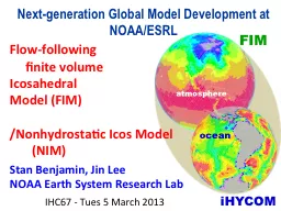
Next-generation Global Model Development at NOAA/ESRL
Flow-following finite volumeIcosahedral Model (FIM)/Nonhydrostatic Icos Model (NIM)
Stan Benjamin, Jin LeeNOAA Earth System Research Lab
IHC67 - Tues
5 March
2013Slide2
FIM Model Development – testing –
http://
fim.noaa.gov
FIM
iHYCOM
atmosphere
ocean
i
HYCOM
– Icosahedral Hybrid Coordinate Ocean Model
Matched grid design to
FIM
for coupled ocean- atmosphere prediction system
Experimental
testing at
ESRL, Navy development
Testing of coupled FIM/
iHYCOM
– toward experimental NMME contribution
FIM – Flow-following finite volume Icosahedral Model
“
soccer-ball
”
grid design for uniform grid
spacing
Isentropic/sigma hybrid vertical coordinate
New 7-14-
day forecast twice
daily
10km
, 15km
, 30km, 60km
Grids to NCEP for evaluation
Real-time experimental at ESRL
Slide3
FIM
global modeldevelopment at NOAA/ESRL and NCEP
Horizontal grid – icosahedral (largely hexagons)
Vertical grid – hybrid isentropic-sigma ResolutionReal-time testing at 60km, 30km,
15km, 10km resolution - icosahedral horizontal grid64 vertical levels – hybrid θ-σ
Ptop = 0.5 hPa,
-top = 2200KPhysicsCurrently GFS physics suite (2011
version)Testing with WRF (Grell
cumulus, PBL)
Initial conditions
GFS/GSI spectral data to FIM
icos
hybrid
θ-σ
vertical coordinate
Ensemble
Kalman
data assimilation in development using FIM model (using NOAA GSI-ensemble code)
Slide4
FIM global model
Horizontal grid
Icosahedral, Arakawa A grid – testing 60km/30km/15km
Vertical grid
Staggered Lorenz grid, ptop = 0.5 hPa, θtop
~2200KGeneralized vertical coordinateHybrid θ-σ option (64L)
GFS σ-p option (64 levels)NumericsAdams-Bashforth 3rd
order time differencingFlux-corrected transport, finite-volumePhysicsGFS physics suite, WRF-Grell cumulus
Coupled model extensionsChem – WRF-chem/GOCARTOcean – icosahedral HYCOMGPU/MIC capability – dynamics complete, physics within 6 mosSlide5
FIM
NIM
global model – non-hydrostatic
incl <5kmHorizontal gridIcosahedral, Arakawa A grid – testing 60km/30km/15kmVertical grid
Staggered Lorenz gridVertical coordinateSigma-z option (
64L)NumericsAdams-Bashforth 3rd
order time differencingFlux-corrected transport, finite volumePhysicsGFS physics suite, GRIMS (Korea mesoscale) suite
Coupled model extensionsChem – WRF-chem/GOCART - futureOcean – icosahedral HYCOM - futureGPU/MIC capability – dynamics complete, physics within 6 mosSlide6
ENDgame
- UKMO
ICON-
IAP – Germany - DWD
MPAS/
G5 - NCAR
NIM/
G5 - ESRL
DCMIP – Dynamic Core Model
Intercomparison
Project:
Experiment 2.1 (non-hydrostatic mountain wave - small
earth
)Slide7
FIM vs. GFS using ECMWF as verification
- Tropical windshttp://www.emc.ncep.noaa.gov/gmb/wx24fy/fimy/ Green
FIM more accurate than GFSSlide8
FIM vs. GFS – 500
hPa AC - Jan-July 2012
N. HemisphereS. HemisphereSlide9
72h forecasts vs.
raobs
N. Hemisphere 20-80N
FIM
vs.
GFS - 2013(FIM lower rms errors for V, T, RH at all levels, similar results at 24h,48h)
FIM better
GFS better
FIM better
GFS better
FIM better
GFS betterSlide10
Resolution
Init
conds
Physics
Diffusion
FIM
30km
GFS
oper
GFS (May 2011,
not May 2012
)
2
nd
-order
FIM9
15km
GFS
oper
GFS
2
nd
-order
FIM9 -
zeus
15km
GFS
oper
GFS
4
th
-order
FIM95
(Jan13)
10km
GFS-ESRL
GFS
2
nd
-order
FIMX
3
0km
GFS
oper
GFS
+
WRF-
chem
, testing of
Grell
cu
2
nd
-order
FIM7
60km
GFS
oper
GFS
2
nd
-order
Versions of FIM
in real-time runs
–
Fall
2012 –
currentSlide11
FIM track forecast skill for 60km, 30km, 15km
versions - 2012 - no other differencesImproved track skill with higher resolution for LANT and EPAC domainsSlide12
Full 2012 track errors – Atlantic +
E.Pacific basinsSlide13
FIM9
Isaac forecasts from HFIP
13Slide14
FIM9 – HFIP – Stream 1.5
FIM9 – ESRL DA
Sandy track forecasts14
Hurricane Sandy forecasts – FIM9 (15km) runs - comparisons with 2 sets of initial conditions1) GFS-operational T574 hybrid DA
(used in FIM9 real-time runs for HFIP) 2) ESRL T878 GFS-EnKF/hybrid DASlide15
HFIP
ESRL-DA
Sandy – initial time 25 Oct 00z
15Slide16
FIM9-DA-HYBUsed ESRL experimental higher-resolution GFS hybrid/
EnKF data assimilation for IC
00z 25 October
Init time runs 120h
132hSlide17
00z 25 October
Init
time runs 120h
132h
FIM9-DA-HYBUsed ESRL experimental higher-resolution GFS hybrid/EnKF data assimilation for ICSlide18
Episodic Weather Extremes from Blocking
Longer-term weather anomalies from atmospheric blocking -Defined here as either ridge or trough quasi-stationary events with duration of at least 4 days to 2+ months
Lead - Stan BenjaminNOAA Earth System Research LaboratoryBoulder, CO
ESPC demo #1 T
arget: improved 1-6 month forecasts of blocking and related weather extremes18Other ESPC Demo #1 team members
Wayne Higgins Randy Dole Shan Sun Melinda PengArun Kumar Judith Perlwitz Rainer Bleck Mingyue
Chen Marty Hoerling John Brown Kathy Pegion Mike Fiorino Slide19
Outcomes from prolonged blocking events or persistent anomalies
FloodingDroughts, excessive firesHeat wave or cold waveExcessive or season-long absent snow cover Excessive ice cover or absence of normal ice cover (example: Great Lakes – 2011-12 winter)Human and economic impact increases exponentially with duration of blocking event
19Slide20
Extratropical wave interaction
MJO life cycleOther tropical processes/ENSOTrop storms, extratrop transitions
Sudden strato warming eventsSnow/ice cover anomaliesSoil moisture anomalies
Initial value – data assim
High-res ΔxCoupled oceanStochastic physics
PV cons. NumericsChem/aerosolSoil/snow LSM accuracy
Processes related to
blocking for
onset, maintenance, cessation
NWP c
omponents
needed
20Slide21
Percentage of blocked days
NCEP GFS – 1-15 day fcstsDec 2011 – March 201221
7
-day GFS forecast blocking frequency is about 50
% of observed7
-day FIM 60km forecast blocking frequency is about 80% of observedSlide22
22
15km
30km
60kmBlocking Strength (
m/deg lat) – FIM 30-day forecasts
ObservedObservedSlide23
23
72h forecastValid 12z 30 Oct Potential temp on PV =2 surface
15km FIM modelSlide24
ESPC Blocking Demo #1 initial findings
Lower blocking frequency in weather and climate models compared to observedKnown problem, worthy of ESPC Demo #1 effort, critical for improved subseasonal-seasonal forecastsInitial 30-day blocking tests with FIMMuch higher blocking frequency than GFS Hypothesis: due to numerical differencesIndependent of resolution
(15km, 30km, 60km)Block duration sensitive to model diffusion and res for FIMEfforts have just barely started
24Slide25
ESPC Demo #1 directions (2013-18)
Hypothesis: Blocking deficiencies may be addressable through improved coupled models (numerics, resolution, physics)What’s new: next-generation global AMIP/CMIP models (higher resolution, modified numerics, readying for GPU/MIC computational era) Expand laboratory links for planned collaboration for blocking research topics for prediction over 1
-26 week durationBuild on NMME community operational ties, also labs with WWRP/ WCRP/THORPEX research “Subseasonal to Seasonal
Prediction Research Implementation Plan25Slide26
ESRL/NOAA plans on
global modelingComplete FIM-EnKF-GSI data assimilation, 4densvar
Improved numerics/physics (PBL, ocean)GEFS experimental FIM testing (plan with NCEP) NMME
experimental testing – coupled FIM- FIM/iHYCOM coupled model (more at GODAE mtg)HFIP (tropical cyclone)
real-time forecasts – 15km, 25km ensembleFIM-chem/CO2/volcanic ash earth system appsNIM real-data testsApplication of FIM/GFS/advanced data assimilation but also NIM and MPAS in
NOAA Research-Regular Pilot Test (also toward HFIP, ESPC goals)