
3 8600 GEOS 28600 Lecture 12 Monday 20 Feb 2017 Fluvial sediment transport introduction REVIEW OF REQUIRED READING SCHOOF amp HEWITT 2013 TURBULENT VELOCITY PROFILES INITIATION OF MOTION ID: 542755
Download Presentation The PPT/PDF document "GEOS" is the property of its rightful owner. Permission is granted to download and print the materials on this web site for personal, non-commercial use only, and to display it on your personal computer provided you do not modify the materials and that you retain all copyright notices contained in the materials. By downloading content from our website, you accept the terms of this agreement.


Slide1
GEOS 38600/ GEOS 28600
Lecture 12
Monday 20 Feb 2017
Fluvial sediment transport: introductionSlide2
REVIEW OF REQUIRED READING (SCHOOF & HEWITT 2013)
TURBULENT VELOCITY PROFILES, INITIATION OF MOTION
BEDLOAD, RIVER GEOMETRY
Fluvial sediment transport: introductionSlide3
Re << 1
inertial forces unimportant Stokes flow / creeping flow:
Schoof & Hewitt 2013
Ice sheets can have multiple stable
equilibria
for the same external forcing, with geologically
rapid transitions between
equilibriaSlide4
Key points from today’s lecture
Critical Shields stress
Differences between gravel-bed vs. sand-bed riversDischarge-width scalingSlide5
Prospectus: fluvial processes
Today: overview, hydraulics, initiation of motion, channel width adjustment.
Channel long-profile evolution.Mountain belts.Final lectures: landscape evolution (including fluvial processes.)This section of the course draws on courses by W.E. Dietrich (Berkeley),D. Mohrig (MIT
U.T. Austin), and J. Southard (MIT).
Slide6
REVIEW OF REQUIRED READING (SCHOOF & HEWITT 2013)
TURBULENT VELOCITY PROFILES, INITIATION OF MOTION
BEDLOAD, RIVER GEOMETRY
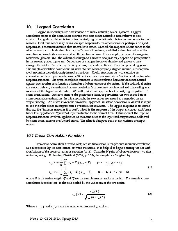
Fluvial sediment transport: introductionSlide7
Hydraulics and sediment transport in rivers:
1) Relate flow to frictional resistance so can relate discharge to hydraulic geometry.
2) Calculate the boundary shear stress.
Parker
Morphodynamics
e-book
pool
Simplified geometry:
average over a
reach
(12-15 channel widths).
we can assume accelerations are zero.
this assumption is better for flood flow (when most of the erosion occurs).
riffle
riffle
poolSlide8
The assumption of no acceleration requires that gravity balances pressure gradients.
Dingman
, chapter 6τ
zx
=
ρgh
sinθaveraging over 15-20 channel widths
forces the water slope to ~ parallel the
basal slopeSlide9
τ
zx
=
ρgh
sinθ
At low slope (S, water surface rise/run),
θ
~ tan
θ
~ sin
θ
τ
b
=
ρgh
S
0
τb1z/h0Frictional resistance:
L
w
h
Boundary stress =
ρgh sinθ L wFrictional resistance = τ
b
L (w + 2 h)
ρgh
sinθ
L
w =
τ
b
L (w + 2 h)
τ
b
=
ρgh
( w / (w + 2 h ) )
sinθ
Define hydraulic radius, R =
hw
/ (w + 2 h)
τ
b
=
ρgR
sin
θ
Basal shear stress, frictional resistance, and hydraulic radius
In very wide channels, R
h (w >> h)Slide10
Law of the wall, recap:
τ
zx =
ρ
K
T
(du/
dz)
τ
zx
=
μ(
T,σ
)
(du/
dz
)
Glaciers ( Re << 1):
Rivers ( Re >> 1, fully turbulent):
eddy viscosity, “diffuses” velocityKT = (k z )2 (du/dz)From empirical & theoretical studies: τB = ρ(k z)2 (du/dz)2 (τB /ρ )1/2 = k z (du / dz) = u* = “shear velocity” (ρ g h S /ρ )1/2 = u* = ( g h S )1/2 Now u* = k z (du / dz)
Separate variables: du = (u* / k z )
dz
Integrate: u = (u*/k) (ln z + c). For convenience, set c = -ln(z0)Then, u = (u*/k) ln
(z/z0)
(where k = 0.39-0.4 = von Karman’s constant)
“law of the wall”
(explained on next slide)
when z = z
0
, u = 0 m/s.
Memorize this.
Properties of turbulence:
Irregularity
Diffusivity
Vorticity
DissipationSlide11
Calculating river discharge, Q (m
3
s-1)z0 is a length scale for grain roughnessvaries with the size of the bedload. In this class, use
z
0
= 0.12 D
84
, where D
84 is the 84thpercentile size in a pebble-count (100th
percentile is the biggest).
Q = <u> w h
<u> = u(z)
dz
(1/(h-z
0
))
z
0
h
<u> = (u*/k) (z0 + h (
ln
( h / z0 ) – 1 ) ) (1/ (h - z0))brackets denote vertical averageu = (u*/k) ln (z/z0)“law of the wall”<u> = (u*/k) ln ( h / e z0) <u> = (u*/k) ln (0.368 h / z0) <u> = (u*/k) ( ln( h / z0 ) – 1 ) h >> z0:typically rounded to 0.4
Extending the law of the wallthrough the flow is a rough
approximation – do not usethis for civil-engineeringapplications. This approachdoes not work at all when
depth clast grainsize.Slide12
Drag coefficient for bed particles:
τB = ρgRS = CD ρ <u>2 / 2
<u> = ( 2g R S / C
D
)
1/2
( 2g / C
D
)
1/2
= C =
Chezy
coefficient
<u> =
C (
R
S
)
1/2
Chezy equation (1769)<u> = ( 8 g / f )1/2 ( R S )1/2f = Darcy-Weisbach friction factor<u> = R2/3 S1/2 n-13 alternative methodsn = Manning roughness coefficient0.025 < n < 0.03 ----- Clean, straight rivers (no debris or wood in channel) 0.033 < n < 0.03 ----- Winding rivers with pools and riffles0.075 < n < 0.15 ----- Weedy, winding and overgrown riversn = 0.031(D84)1/6 ---- Straight, gravelled riversIn sand-bedded rivers (e.g. Mississippi), form drag due to sand dunes is important.In very steep streams, supercritical flow may occur:Froude numberFr
# = <u>/(gh)1/2 > 1
supercritical flow
Most used, because lots of investment in measuring n for different objectsSlide13
John SouthardSlide14
Sediment transport in rivers:
(Shields number)
F
D
F
L
F’
g
(submerged weight)
Φ
At the initiation of grain motion,
F
D
= (
F’
g
– F
L
) tan
Φ
FD/F’g =tan Φ 1 + (FL/FD) tan Φ ≈ τc D2
(
ρ
s – ρ)gD3 =
τc =
τ*
(
ρ
s
–
ρ
)
gD
Shields number (“drag/weight ratio”)
Is there a representative particle size for the
bedload
as a whole?
Yes: it’s D
50
.Slide15
Equal mobility hypothesis
F
D
F
L
F’
g
(submerged weight)
Φ
Φ
D/D
50
“Hiding” effect
small particles
don’t move significantly
before the D
50
moves.
Significant controversy over validity of equal mobility hypothesis in the late
’
80s – early
’
90s.
Parameterise
using
τ
*
= B(D/D
50
)
α
α = -1 would indicate perfect equal mobility (
no
sorting by grain size with downstream distance)
α =
-0.9 found from flume experiments (permitting long-distance sorting by grain size).
Trade-off between size and
embeddednessSlide16
Buffington & Montgomery, Water Resources Research, 1999
sand
gravel
τ
*c50
~ 0.04, from experiments
(0.045-0.047 for gravel, 0.03 for sand)
1936:
1999:
Theory has approximately
reproduced some parts
of this curve.
Causes of scatter:
(1) differing definitions of
initiation of motion (most important).
(2) slope-dependence?
(Lamb et al. JGR 2008)
Hydraulically rough:
viscous
sublayer
is a thin
skin around the particles.Re* = “Reynolds roughness number”Slide17
REVIEW OF REQUIRED READING (SCHOOF & HEWITT 2013)
TURBULENT VELOCITY PROFILES, INITIATION OF MOTION
BEDLOAD, RIVER GEOMETRY
Fluvial sediment transport: introductionSlide18
Consequences of increasing shear stress: gravel-bed vs. sand-bed rivers
John Southard
Suspension: characteristic velocity forturbulent fluctuations (u*) exceeds
settling velocity (ratio is ~Rouse number).
Typical transport distance
100m/
yr
in gravel-bedded
bedload
Sand: km/day
Empirically, rivers are either gravel-bedded or sand-bedded (little in between)
The cause is unsettled: e.g. Jerolmack &
Brzinski
Geology 2010 vs. Lamb &
Venditti
GRL 2016
(Experimentally, u* is approximately
equal to
rms
fluctuations in vertical
turbulent velocity)Slide19
Bedload transport
(Most common
:) qbl = kb(
τ
b
–
τ
c
)3/2
there is no theory for
washload
:
it is entirely controlled by upstream supply
Many alternatives, e.g.
Yalin
Einstein
Discrete element modeling
John Southard
Meyer-Peter MullerSlide20
River channel morphology and dynamics
“Rivers are the authors of their own geometry” (L. Leopold)
And of their own bed grain-size distribution.Rivers have well-defined banks.Bankfull discharge 5-7 days per year; floodplains inundated every 1-2 years.Regular geometry also applicable to canyon rivers.Width scales as Q0.5
River beds are (usually) not flat.
Plane beds are uncommon. Bars and pools, spacing = 5.4x width.
Rivers meander.
Wavelength ~ 11
x
channel width.River profiles are concave-up.Grainsize also decreases downstream.Slide21
>20%;
colluvial
Slope, grain size, and transport mechanism: strongly correlated
z
<0.1%
bar-pool
sand
bedload
& suspension
0.1-3%
bar-pool
gravel
bedload
3-8%
step-pool
gravel
bedload
8-20%
boulder
cascade
(periodically
swept bydebrisflows)rocks may beabraded in place;fine sediment bypasses bouldersSlide22
What sets width?
Eaton, Treatise on
Geomorphology, 2013Q = wd
<u>
w =
aQ
b
d
= cQf
<u> =
kQ
m
b+f+m
= 1
b = 0.5
m = 0.1
f = 0.4
Comparing
different points
downstreamSlide23
(1) Posit empirical relationships between hydraulics, sediment supply, and form
(Parker et al. 2008 in suggested reading; Ikeda et al. 1988 Water Resources Research).
(2) Extremal hypotheses; posit an optimum channel, minimizing energy (Examples: minimum streampower per unit length; maximum friction; maximum sediment transport rate; minimum total streampower; minimize Froude number)(3) What is the actual mechanism? What controls what sediment does, how high the bank is, & c.?
What sets width? Three approaches to this unsolved question: Slide24
Key points from today’s lecture
Critical Shields stress
Differences between gravel-bed vs. sand-bed riversDischarge-width scaling