Figure 1. Sketch of the axisymmetric case ( - PowerPoint Presentation

Slide1

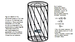
Figure 1. Sketch of the axisymmetric case (

m

= 0) tube structure. Twisted field lines are shown. The inward force associated with the field curvature is balanced by the combination of radial magnetic field pressure and the centripetal acceleration associated with the rotation. The inner cylinders illustrate the contours of pressure.

Even in perfectly compressible (cold) or incompressible limits this configuration can only be achieved by a radial pressure gradient balancing centripetal acceleration.

As in steady state

In fact, the situation represents the

column rotating exactly as if it were

a rigid body!

The only fluid effect is that the radial

pressure gradient balances

centripetal effects. Slide2

a

b

c

dSlide3

(a)

(b)

m

= 0 field aligned

current distribution

m

= 0 flow

pattern

Figure 2. Cross-section of the plasma column once

steady rotation

has

started,

in the axisymmetric (

m

= 0) case. The magnetic field is assumed to be into the page. (a) illustrates the distribution of field aligned current. A surface current on the outer boundary shields the exterior from the twisted field. Current flows horizontally through the conductor. The return field aligned current is distributed across the cross-section. The overall current system is closed in the travelling front which originally brings the column into rotation. (b) shows the flow. Slide4

Figure

5. Illustration of a field line displaced by the wave. The line in question lies on the boundary of the cylinder. An unperturbed field line is illustrated by the dotted straight line. The perturbed field line passes through the points

a, b, c, d, and e. From a to

c the line is on the near side of the cylinder. From c to e the line is on the far side of the cylinder and is shown dashed. In one wave length (as illustrated) it does a complete circuit of the tube. With a right handed rotation at the base, the field makes a left handed spiral up the tube. Because of the polarisation reversal across the cylinder surface, the field lines outside make a right hand spiral (not shown). On the distorted column boundary where the spiral sense reverses field aligned current flows.Slide5
Slide6

Energy issues

Working to linear order in the amplitude of the disturbance on the background, the energy per unit length is second order,

There is

equi

-partition also in the

m = 1, case (cf. Walen relation) so one may also write

As  can be vanishingly small, comparing 4’ and 3’, shows that the energy required to set up the

m = 1 configuration is less than that required to set up the m = 0 configuration as long as the displacement is much less than the column radius, a. In fact, the size of  is determined by storage/transmission of angular momentum the boundary condition along the field as the angular momentum stored is proportional to 2. The m = 1 mode can be precluded if it is suppressed in some way. For example, if the boundary at r = a were rigid and so radial motion there were impossible. Such a rigid boundary would impose a compressional

m = 0 structure. The rigid boundary example is an extreme case. The m = 0 mode is confined to the column whereas m = 1 includes a thin exterior region. (3)(4)(4’)Now there is equipartition between transverse components of velocity and field (i.e. bf ) in (1) due to the Walen relation

(3’)Slide7

Energy issues

Working to linear order in the amplitude of the disturbance on the background, the energy per unit length is second order,

There is

equi

-partition also in the

m = 1, case (cf. Walen relation) so one may also write

(3)

(4)Now there is equipartition between transverse components of velocity and field (i.e. bf ) in (1) due to the Walen relation

(3’)Slide8

Instantaneous streamlinesSlide9

Southwood and Cowley 2014 Slide10

?

?

Flux with solar wind entry

Flux with solar wind entrySlide11

Figure 3. Illustration of the column cross-section distorted by the wave fields in the

m = 1 mode. The continuous lines represent the instantaneous transverse field or flow lines. The continuous circle indicates the undisturbed original column boundary and the dashed line, the boundary which is now displaced

by the wave. The sketch illustrates that the interior flow is at right angles to the peak displacement. The rotation at the base of the column imposes a cam-like motion in which the displacement at all points is the same. The pattern not only rotates, as the curved arrow indicates, with time but also with along the column with varying z thus producing the kink motion.

For

m

=

1, an purely incompressible response is

possible ( = plasma displacement) Along the field the wave structure is governed by the Alfvén wave dispersion relation

(1)For m = 1, equation (1) yields

r < ar > aand

The capacity for radial motion at the column boundary is fundamental for this mode (and all m ≠ 0 modes). Radial motion is also needed at the base. This is not a problem when the “base” is the open-closed field line boundary (or something similar) – and is seen in the Saturn aurora (Nichols et al.).[Anyone who has skipped with a jump rope is (perhaps unconsciously) aware of the effect.] Slide12

Figure 7

Figure

4.

Structure of wave

fields in the

m

=1 case. In the centre, the column is shown distorted by the wave fields. The wave propagates in the direction of the background field and is left hand polarised with respect to B (in the z‑direction. On the far left are shown the instantaneous flow in the plane transverse to the column, then is sketched the distortion of the column in (x, y) with continuous/dashed lines indicating the undisplaced/displaced cross-sections respectively at different positions along the column. On the right are shown sketches of the perpendicular current and the associated j 

 B force. Slide13
Slide14

Angular momentum issues

Working to linear order in the amplitude of the disturbance on the background, the angular momentum density in the m = 0 case is,

The above lays bare the difference between the “rigid body”

m

= 0 rotation and the m

= 1 (kink mode). The plasma displacement  can be vanishingly small and, in practice, the amplitude  of the m = 1 configuration can be tuned to provide any angular momentum density. Moreover, as the signal is time varying and looks like a traveling wave angular momentum can be carried continuously from the base up the column along the field.

In fact, the size of  is determined by storage/transmission of angular momentum the boundary condition along the field as the angular momentum stored is proportional to 2. Moreover, the m = 1 carries a flux of angular momentumwhich can be tuned arbitrarily. In contrast, although there is angular momentum stored in the m = 0, switching on rotation from below results in a front traveling up the tube which brings the tube into full rigid rotation (and modifies field pressure to balance the radial centrifugal stress). There is angular momentum stored behind the front but no continuous flux. (1)

(2)(2’)Thus the angular momentum stored per unit length in the rotating column is (1’)

In contrast the angular momentum in the m = 1 case is uniformly distributed across the column Slide15

Presssure contoursSlide16

Figure

6. Comparison of the field aligned sheet currents on the edge of the flux tube treading the obstacle in a) the familiar obstacle in flow case and b) the case of a rotating source embedded in a plasma and emitting m

 = 1 kink waves that is introduced in this paper. On the surface reversed field aligned currents form on each flank with strength varying sinusoidally in azimuth. The sheet currents are indicated by the positive (+z direction) and negative signs (‑z direction). Flow lines associated with the wave in the frame of the obstacle are sketched in each case. The patterns are similar. However, in case b) everything rotates with angular velocity,

W, and the cross-section itself is displaced at right angles to the transverse flow inside the tube. Slide17

Figure 7.

Alfvén mode wings and rotating kink modes contrasted once more. Sketch (a) shows a cross-section in the (x, z) plane containing the field and flow velocity. Sketch (b) shows the projection in the (

y, z) plane containing the field and transverse to the flow. Sketches (c) and (d) show the equivalent characteristics for the case of a steadily rotating obstacle embedded in a stationary plasma. The structure is stationary in the frame of the rotating object. The current carrying structure spirals away from the object and so the projections in the (x, z) and (

y, z) planes are in spatial quadrature (as sketched). Slide18

Figure 8. Sketch of a rotating magnetised body where the polar cap field lines are open. The sense of rotation is indicated by the broad arrows. The dotted boundary on the object marks the open-closed field boundary on the body. Open field lines at the boundary are sketched. The field lines spiral and with the same convention as Figure 4 continuous traces show segments on the viewers side of the tube and dashed lines indicate the trace behind. The polar cap flux tube cross-section increases with radial distance. The degree of kinking depends on the angular momentum transfer. However, independent of whether the internal field of the body is axially symmetric or not, under all circumstances kinking is necessary for momentum transmission. Slide19
Slide20

N

S

Answering the

Krishan

Khurana

question (why the tail wags the dog)

Imagine a steady

In flux of solar windSlide21

In northern winter the northern cusp entry layer presents a smaller cross-section to the solar wind.

In northern winter, more solar wind particles would access southern cusp/entry layer – adding inertia to rotation of southern cap.

The northern winter, slower southern rotation is than the northern is likely due to the differential access to and then loading of cusp/entry layer

If the seasonal rotation differential were due to differential illumination, in northern winter the northern cap would rotate faster than the southern.

NOT SEENSlide22

N

S

Equinoctial Oscillations

Imagine a steady

In flux of solar windSlide23

N

S

Equinoctial Oscillations

Imagine a steady

In flux of solar windSlide24

N

S

Equinoctial Oscillations

Imagine a steady

In flux of solar windSlide25

S

N

Equinoctial Oscillations

Imagine a steady

In flux of solar windSlide26

S

N

Equinoctial Oscillations

Imagine a steady

In flux of solar windSlide27

S

N

Equinoctial Oscillations

Imagine a steady

In flux of solar windSlide28

N

S

Equinoctial Oscillations

Imagine a steady

In flux of solar windSlide29

N

S

Equinoctial Oscillations

Imagine a steady

In flux of solar windSlide30

N

S

Equinoctial Oscillations

Imagine a steady

In flux of solar windSlide31

N

S

Equinoctial Oscillations

Imagine a steady

In flux of solar windSlide32

N

S

Equinoctial Oscillations

Imagine a steady

In flux of solar windSlide33

S

N

Equinoctial Oscillations

Imagine a steady

In flux of solar windSlide34

S

N

Equinoctial Oscillations

Imagine a steady

In flux of solar windSlide35

S

N

Equinoctial Oscillations

Imagine a steady

In flux of solar windSlide36

N

S

Equinoctial Oscillations

At equinox, periods north and south should be similar

however recall the offset dipole and so northern cusp is closer to pole at actual equinox – south should dominate

Immediately post-equinox, can envisage chaotic switching

Once southern winter in full swing northern should dominate and be slower –

Prediction!!

Imagine a steady

In flux of solar windSlide37
Slide38
Slide39
Slide40

Outflow down tail

(“planetary” wind)

X X X X X X X X X X X

X X X X X

Return flow of accelerated

residual solar wind material

Vasyliunas

regime

(confined near equator

slowly rotating)Slide41
Slide42
Slide43