
Bias Variance Tradeoff Guest Lecturer Joseph E Gonzalez s lides available here httptinyurlcom reglecture Simple Linear Regression Y X Linear Model Response Variable Covariate Slope ID: 1022948
Download Presentation The PPT/PDF document "Linear Regression and the" is the property of its rightful owner. Permission is granted to download and print the materials on this web site for personal, non-commercial use only, and to display it on your personal computer provided you do not modify the materials and that you retain all copyright notices contained in the materials. By downloading content from our website, you accept the terms of this agreement.


1. Linear Regression and the Bias Variance TradeoffGuest LecturerJoseph E. Gonzalezslides available here: http://tinyurl.com/reglecture
2. Simple Linear RegressionYXLinear Model:ResponseVariableCovariateSlopeIntercept (bias)
3. MotivationOne of the most widely used techniquesFundamental to many larger modelsGeneralized Linear ModelsCollaborative filteringEasy to interpretEfficient to solve
4. Multiple Linear Regression
5. The Regression ModelFor a single data point (x,y):Joint Probability:Response Variable(Scalar)Independent Variable(Vector)xyxObserve:(Condition)Discriminative Model
6.
7. The Linear ModelScalarResponseVector of CovariatesReal ValueNoiseNoise Model:What about bias/intercept term?Vector ofParametersLinear Combination of CovariatesThen redefine p := p+1 for notational simplicity+ b
8. Conditional Likelihood p(y|x)Conditioned on x:Conditional distribution of Y:ConstantNormal DistributionMeanVariance
9. ParametersParameters and Random VariablesConditional distribution of y:Bayesian: parameters as random variablesFrequentist: parameters as (unknown) constants
10. *YX2X1I’m lonelySo far …
11. Plate DiagramIndependent and Identically Distributed (iid) DataFor n data points:Response Variable(Scalar)Independent Variable(Vector)xiyi
12. Joint ProbabilityFor n data points independent and identically distributed (iid):xiyi
13. Rewriting with Matrix NotationRepresent data as:npCovariate (Design)Matrixn1ResponseVectorAssume X has rank p(not degenerate)
14. Rewriting with Matrix NotationRewriting the model using matrix operations:npn11pn= +
15. Estimating the ModelGiven data how can we estimate θ?Construct maximum likelihood estimator (MLE):Derive the log-likelihood Find θMLE that maximizes log-likelihoodAnalytically: Take derivative and set = 0Iteratively: (Stochastic) gradient descent
16. Joint ProbabilityFor n data points:xiyiDiscriminative Modelxi“1”
17. Defining the Likelihoodxiyi
18. Maximizing the LikelihoodWant to compute:To simplify the calculations we take the log:which does not affect the maximization because log is a monotone function.
19. Take the log:Removing constant terms with respect to θ:Monotone Function(Easy to maximize)
20. Want to compute:Plugging in log-likelihood:
21. Dropping the sign and flipping from maximization to minimization:Gaussian Noise Model Squared LossLeast Squares RegressionMinimize Sum (Error)2
22. Pictorial Interpretation of Squared Erroryx
23. Maximizing the Likelihood(Minimizing the Squared Error)Take the gradient and set it equal to zeroSlope = 0Convex Function
24. Minimizing the Squared ErrorTaking the gradientChain Rule
25. Rewriting the gradient in matrix form:To make sure the log-likelihood is convex compute the second derivative (Hessian)If X is full rank then XTX is positive definite and therefore θMLE is the minimum Address the degenerate cases with regularization
26. NormalEquations(Write on board)Setting gradient equal to 0 and solve for θMLE:p-1=pnn1
27. Geometric InterpretationView the MLE as finding a projection on col(X)Define the estimator:Observe that Ŷ is in col(X)linear combination of cols of XWant to Ŷ closest to YImplies (Y-Ŷ) normal to X
28. Connection to Pseudo-InverseGeneralization of the inverse:Consider the case when X is square and invertible:Which implies θMLE= X-1 Y the solution to X θ = Y when X is square and invertible Moore-Penrose Psuedoinverse
29. or use the built-in solver in your math library.R: solve(Xt %*% X, Xt %*% y)Computing the MLENot typically solved by inverting XTXSolved using direct methods:Cholesky factorization:Up to a factor of 2 fasterQR factorization:More numerically stableSolved using various iterative methods:Krylov subspace methods(Stochastic) Gradient Descenthttp://www.seas.ucla.edu/~vandenbe/103/lectures/qr.pdf
30. Cholesky FactorizationCompute symm. matrixCompute vector Cholesky Factorization L is lower triangularForward subs. to solve: Backward subs. to solve: CdConnections to graphical model inference: http://ssg.mit.edu/~willsky/publ_pdfs/185_pub_MLR.pdf and http://yaroslavvb.blogspot.com/2011/02/junction-trees-in-numerical-analysis.html with illustrations
31. Solving Triangular System=*A11A12A13A14A22A23A24A33A34A44b1b2b3b4A11x1A12x2A13x3A14x4x1x2x3x4Bonus Content
32. Solving Triangular SystemA11x1A12x2A13x3A14x4A22x2A23x3A24x4A33x3A34x4A44x4b1b2b3b4x4=b4 /A44x3=(b3-A34x4) A33x2=b2-A23x3-A24x4 A22x1=b1-A12x2-A13x3-A14x4 A11Bonus Content
33. Distributed Direct Solution (Map-Reduce)Distribution computations of sums:Solve system C θMLE = d on master.ppp1
34. Gradient Descent: What if p is large? (e.g., n/2)The cost of O(np2) = O(n3) could by prohibitiveSolution: Iterative MethodsGradient Descent:For τ from 0 until convergenceLearning rate
35. Slope = 0Gradient Descent Illustrated:Convex Function
36. Gradient Descent: What if p is large? (e.g., n/2)The cost of O(np2) = O(n3) could by prohibitiveSolution: Iterative MethodsGradient Descent:Can we do better?For τ from 0 until convergenceEstimate of the Gradient
37. Stochastic Gradient DescentConstruct noisy estimate of the gradient:Sensitive to choice of ρ(τ) typically (ρ(τ)=1/τ)Also known as Least-Mean-Squares (LMS)Applies to streaming data O(p) storageFor τ from 0 until convergence 1) pick a random i 2)
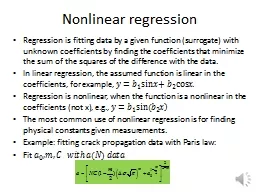
38. Fitting Non-linear DataWhat if Y has a non-linear response?Can we still use a linear model?
39. Transforming the Feature SpaceTransform features xiBy applying non-linear transformation ϕ:Example:others: splines, radial basis functions, …Expert engineered features (modeling)
40. Under-fittingOver-fitting
41. Really Over-fitting!Errors on training data are smallBut errors on new points are likely to be large
42. What if I train on different data?Low Variability:High Variability
43. Bias-Variance TradeoffSo far we have minimized the error (loss) with respect to training dataLow training error does not imply good expected performance: over-fitting We would like to reason about the expected loss (Prediction Risk) over:Training Data: {(y1, x1), …, (yn, xn)}Test point: (y*, x*)We will decompose the expected loss into:
44. Define (unobserved) the true model (h):Completed the squares with:abExpected LossAssume 0 mean noise[bias goes in h(x*)]
45. Define (unobserved) the true model (h):Completed the squares with:Substitute defn. y* = h* + e*Expected Loss
46. ExpandDefine (unobserved) the true model (h):Completed the squares with:Minimum error is governed by the noise.Noise Term(out of our control)Model Estimation Error(we want to minimize this)Expected Loss
47. Expanding on the model estimation error:Completing the squares with
48. Expanding on the model estimation error:Completing the squares with
49. Expanding on the model estimation error:Completing the squares withTradeoff between bias and variance:Simple Models: High Bias, Low VarianceComplex Models: Low Bias, High Variance(Bias)2Variance
50. Summary of Bias Variance TradeoffChoice of models balances bias and variance.Over-fitting Variance is too HighUnder-fitting Bias is too HighExpected LossNoise(Bias)2Variance
51. Bias Variance PlotImage from http://scott.fortmann-roe.com/docs/BiasVariance.html
52. Assume a true model is linear:Plug in definition of YExpand and cancelSubstitute MLEAssumption:is unbiased!Analyze bias of
53. Assume a true model is linear:Use property of scalar: a2 = a aTAnalyze Variance of Substitute MLE + unbiased resultPlug in definition of YExpand and cancel
54. Use property of scalar: a2 = a aTAnalyze Variance of
55. Consequence of Variance CalculationHigher VarianceLower VarianceFigure from http://people.stern.nyu.edu/wgreene/MathStat/GreeneChapter4.pdf
56. Analyze Variance of Assume a true model is linear:Next: use matrix variance identitySubstitute MLE + unbiased resultPlug in definition of YExpand and cancel
57. Analyze Variance of Define:Use matrix variance identity:If we assume x is iid N(0, 1):
58. Deriving the final identityAssume xi and x* are N(0,1)
59. SummaryLeast-Square Regression is Unbiased:Variance depends on:Number of data-points nDimensionality pNot on observations Y
60. Gauss-Markov TheoremThe linear model:has the minimum variance among all unbiased linear estimatorsNote that this is linear in YBLUE: Best Linear Unbiased Estimator
61. SummaryIntroduced the Least-Square regression modelMaximum Likelihood: Gaussian NoiseLoss Function: Squared ErrorGeometric Interpretation: Minimizing ProjectionDerived the normal equations:Walked through process of constructing MLEDiscussed efficient computation of the MLEIntroduced basis functions for non-linearityDemonstrated issues with over-fittingDerived the classic bias-variance tradeoffApplied to least-squares model
62.
63. Additional Reading I found Helpfulhttp://www.stat.cmu.edu/~roeder/stat707/lectures.pdfhttp://people.stern.nyu.edu/wgreene/MathStat/GreeneChapter4.pdfhttp://www.seas.ucla.edu/~vandenbe/103/lectures/qr.pdfhttp://www.cs.berkeley.edu/~jduchi/projects/matrix_prop.pdf