Chapter 5: Sampling Distributions - PowerPoint Presentation

Slide1

Chapter 5:Sampling Distributions

Lecture Presentation Slides

Macmillan Learning ©

2017Slide2

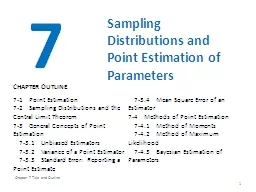
Chapter 5Sampling Distributions

5.1 Toward Statistical Inference5.2 The Sampling Distribution of a Sample Mean5.3 Sampling Distributions for Counts and Proportions

2Slide3

5.1 Toward Statistical InferenceParameters and statistics

Sampling variabilitySampling distributionsBias and variabilitySampling from large populations

3Slide4

Parameters and Statistics

4

As we begin to use sample data to draw conclusions about a wider population, we must be clear about whether a number describes a sample or a population.

A

parameter

is a number that describes some characteristic of the population. In statistical practice, the value of a parameter is not known because we cannot examine the entire population.

A

statistic

is a number that describes some characteristic of a sample. The value of a statistic can be computed directly from the sample data, but it can change from sample to sample. We often use a statistic to estimate an unknown parameter.

Remember

s

and p: statistics come from samples andparameters come from populations.

We write µ (the Greek letter mu) for the population mean and σ for the population standard deviation. We write (x-bar) for the sample mean and s for the sample standard deviation.

 Slide5

Statistical Estimation

5

The process of

statistical inference

involves using information from a sample to draw conclusions about a wider population.

Different random samples yield different statistics

. We need to be able to describe the

sampling distribution

of the possible values of a statistic in order to perform statistical inference.

The sampling distribution of a statistic consists of all possible values of the statistic and the relative frequency with which each value occurs. We may plot this distribution using a histogram, just as we plotted a histogram to display the distribution of data in Chapter 1.

Population

Sample

Collect data

from a representative

Sample...Make an inference about the Population.Slide6

6Slide7

Sampling Variability

7

Sampling variability

is a term used for the fact that the value of a statistic varies in repeated random sampling.

To make sense of sampling variability, we ask,

“

What would happen if we took many samples?

”

Population

Sample

Sample

Sample

Sample

Sample

Sample

Sample

Sample

?Slide8

Sampling Distributions

8

If we measure enough subjects, the statistic will be very close to the unknown parameter that it is estimating.

If we took every one of the possible samples of a certain size, calculated the sample mean for each, and made a histogram of all of those values, we’

d have a

sampling distribution

.

The

sampling distribution

of a statistic is the distribution of values taken by the statistic in all possible samples of the same size from the same population.

In practice, it

is difficult to take all possible samples of size

n

to obtain the actual sampling distribution of a statistic. Instead, we can use simulation to imitate the process of taking many, many samples.Slide9

Bias and Variability

9

We can think of the true value of the population parameter as the bull’s-eye on a target and of the sample statistic as an arrow fired at the target. Bias and variability describe what happens when we take many shots at the target.

Bias

concerns the center of the sampling distribution. A statistic used to estimate a parameter is

unbiased

if the mean of its sampling distribution is equal to the true value of the parameter being estimated.

The

variability of a statistic

is described by the spread of its sampling distribution. This spread is determined by the sampling design and the sample size

n. Statistics from larger probability samples have smaller spreads.Slide10

10Slide11

11Slide12

Managing Bias and Variability

12

A good sampling scheme must have both small bias and small variability.

To reduce bias

, use random sampling.

To reduce variability

of a statistic from an SRS, use a larger sample.

The variability of a statistic from a random sample does not depend on the size of the population, as long as the population is at least 20 times larger than the sample.Slide13

13Slide14

Why Randomize?

14

The purpose of a sample is to give us information about a larger population. The process of drawing conclusions about a population on the basis of sample data is called

inference

.

Why should we rely on random sampling?

To eliminate bias in selecting samples from the list of available individuals.

The laws of probability allow trustworthy inference about the population.

Results from random samples come with a

margin of error

that sets bounds on the size of the likely error.

Larger random samples give better information about the population than smaller samples.Slide15

5.2 The Sampling Distribution of a Sample MeanPopulation distribution

The mean and standard deviation of the sample meanSampling distribution of a sample meanCentral limit theorem

15Slide16

Population Distribution

16

The

population distribution

of a variable is the distribution of values of the variable among all individuals in the population. The population distribution is also the probability distribution of the variable when we choose one individual at random from the population.

In many examples, there is a well-defined population of interest from which SRS’s can be drawn, as when we sample students who attend a particular university.

However, sometimes the population of interest does not actually exist. For example, the exam scores of students who took a course

last

semester can be thought of as a sample from a hypothetical population of students who will take the course in the future, but that population of students does not yet exist. We can still think of the observations as having come from a population with a probability distribution.Slide17

Mean and Standard Deviation of a Sample Mean

17

Mean of a sampling distribution of a sample mean

There is no tendency for a sample mean to fall systematically above or below

m

,

even if the distribution of the raw data is skewed. Thus, the mean of the sampling distribution is an

unbiased

estimate

of the population mean

m.Standard deviation of a sampling distribution of a sample mean

The standard deviation of the sampling distribution measures how much the sample statistic varies from sample to sample. It is smaller than the standard deviation of the population by a factor of √n.  Averages are less variable than individual observations. Slide18

18

FIGURE 5.6 (a) The distribution of visit lengths to a statistics help room during the school year, Example 5.5. (b) The distribution of the sample means (x-bar) for 500 random samples of size 60 from this population. The scales and histogram classes are exactly the same in both panels.Slide19

19Slide20

The Sampling Distribution of a Sample Mean

20

When we choose many SRS’s from a population, the sampling distribution of the sample mean is centered at the population mean

µ

and is less spread out than the population distribution. Here are the facts.

The Sampling Distribution of Sample Means

Suppose that

is the mean of an SRS of size

n

drawn from a large population with mean

and standard deviation

. Then:

The

mean

of the sampling distribution of is

The

standard deviation

of the sampling distribution of

is

If individual observations have the

N

(

µ,σ)

distribution, then the sample mean of an SRS of size

n

has the

N

(

µ

, σ/√

n

) distribution, regardless of the sample size

n

.Slide21

21Slide22

22Slide23

23Slide24

The Central Limit Theorem

24

Most population distributions are not Normal. What is the shape of the sampling distribution of sample means when the population distribution is not Normal?

It is a remarkable fact that,

as the sample size increases, the distribution of sample means begins to look more and more like a Normal distribution!

When the sample is large enough, the distribution of sample means is very close to Normal,

no matter what shape the population distribution has,

as long as the population has a finite standard deviation.Slide25

25Slide26

26Slide27

Central Limit Theorem Example

27

Based on service records from the past year, the time (in hours) that a technician requires to complete preventive maintenance on an air conditioner follows a distribution that is strongly right-skewed and whose most likely outcomes are close to 0. The mean time is

µ

= 1 hour and the standard deviation is

σ

= 1.

Your company will service an SRS of 70 air conditioners. You have budgeted 1.1 hours per unit. Will this be enough?

The mean and standard deviation of the sampling distribution of the average time spent working on the 70 units are

The central limit theorem says that the sampling distribution of the mean time spent working is approximately

N

(1, 0.12) because

n

= 70 ≥ 30.

If you budget 1.1 hours per unit, there is a 20% chance the technicians will not complete the work within the budgeted time.Slide28

5.3 Sampling Distributions for Counts and ProportionsBinomial distributions for sample counts

Binomial distributions in statistical samplingFinding binomial probabilitiesBinomial mean and standard deviation

Sample proportions

Normal approximation for counts and proportions

Binomial formula

Poisson distributions

28Slide29

Bernoulli Random Variable

29

A random variable that has only two outcomes 0 and 1 is called a

Bernoulli

random variable

-- 1 denotes

success

and 0 denotes failure.

Here is the probability table for a Bernoulli random variable:

X

Probability

1

p01 - pSome examples of Bernoulli random variables:

flipping a coin (T = 0, H = 1), rolling an ace with a single die (non-ace = 0, ace = 1), shooting a basketball free throw (failure = 0, success = 1), choosing a part from an assembly line to inspect (non-defective = 0, defective = 1).Slide30

The Binomial Setting

30

When Bernoulli process is repeated several times, we are often interested in whether a particular outcome does or does not happen on each repetition. In some cases, the number of

repeated trials

is fixed in advance, and we are interested in the

number of times

a particular event (called a

“

success

”

) occurs. Slide31

Binomial Distribution

31

Binomial Distribution

The count

X

of successes in a binomial setting has the

binomial distribution

with parameters

n

and

p

, where n is the number of trials of the chance process and p is the probability of a success on any one trial. The possible values of X are the whole numbers from 0 to n.Slide32

32Slide33

Binomial Probability

33

The binomial coefficient counts the number of different ways in which

k

successes can be arranged among

n

trials. The

binomial probability

P

(

X

=

k) is this count multiplied by the probability of any one specific arrangement of the k successes.Binomial Probability

If X has the binomial distribution with n trials and probability p of success on each trial, the possible values of X are 0, 1, 2, …, n. If k is any one of these values:

Number of arrangements of

k

successes

Probability of

k

successes

Probability of

n−k

failuresSlide34

Binomial Coefficient

34

Here, we justify the expression given previously for the binomial distribution. First, we can find the chance that a binomial random variable takes any value by

adding probabilities for the different ways of getting exactly that many successes in

n

observations

.

The number of ways of arranging

k

successes among

n

observations is given by the

binomial coefficient

for k = 0, 1, 2, …, n.Note:

n! = n(n – 1)(n – 2)•…•(3)(2)(1) and 0! = 1. Slide35

35Slide36

Binomial Probability Example

36

Each child of a particular pair of parents has probability 0.25 of having blood type O. Suppose the parents have five children.

(a) Find the probability that exactly three of the children have type O blood.

Let

X

= the number of children with type O blood. We know

X

has a binomial distribution with

n

= 5

and p = 0.25.

(b) Should the parents be surprised if more than three of their children have type O blood?

Since there is only a 1.5% chance that more than three children out of five would have Type O blood, the parents should be surprised!Slide37

37Slide38

38Slide39

39Slide40

Binomial Mean and Standard Deviation

40

Mean and Standard Deviation of a Binomial Random Variable

If a count

X

has the binomial distribution with number of trials

n

and probability of success

p

, the

mean

and standard deviation of X are

Also,  Slide41

41Slide42

Normal Approximation for Binomial Distributions P(X=k)

42

As

n

gets larger, something interesting happens to the shape of a binomial distribution.

Normal Approximation for Binomial Distributions

Suppose that

X

has the binomial distribution with

n

trials and success probability

p

.

When n is large, the distribution of X is approximately Normal with mean and standard deviation

As a rule of thumb, we will use the Normal approximation when n is so large that np ≥ 10 and n(1 – p) ≥ 10.  Slide43

Normal Approximation (Counts) Example

43

Sample surveys show that fewer people enjoy shopping than in the past. A survey asked a nationwide random sample of 2500 adults if they agreed or disagreed that

“

I like buying new clothes, but shopping is often frustrating and time-consuming.

”

Suppose that exactly 60% of all adult U.S. residents would say

“

Agree

”

if asked the same question. Let

X

= the number in the sample who agree. Estimate the probability that 1520 or more of the sample agree.1) Verify that X is approximately a binomial random variable.

B: Success = agree; Failure = do not agreeI: Because the population of U.S. adults is greater than 25,000, it is reasonable to assume that the 2500 trials are independent of each other. N: n = 2500 trials of the chance process.S: The probability of selecting an adult who agrees is p = 0.60.

2) Check the conditions for using a Normal approximation.

Because

np

= 2500(0.60) = 1500 and

n

(1 –

p

) = 2500(0.40) = 1000 are both at least 10, we may use the Normal approximation.

3) Calculate

P

(

X

≥ 1520) using a Normal approximation.Slide44

Binomial (X) to Sample Proportion (

) 

44Slide45

45

Sample Proportion Mean and

StdevSlide46

46Slide47

47

Sampling Distribution of a Sample Proportion

Choose an SRS of size

n

from a population of size

N

with proportion

p

of successes. Let

be the sample proportion of successes. Then:

The

mean

of the sampling distribution is p. The standard deviation of the sampling distribution is

For large n, has approximately the

distribution. As n increases, the sampling distribution becomes approximately Normal. Slide48

Normal Approximation of Binomial Counts and Proportion48

Given that

is approximately Normal, the counts X will also be Normal because it is just a constant n times

.

 Slide49

49Slide50

50Slide51

51

Note: (a) is about sample proportion, while (b) is about Binomial distribution.