Sampling Distributions - PowerPoint Presentation

Slide1

Sampling Distributions

Martina Litschmannová

m

artina.litschmannova

@vsb.cz

EA 538Slide2

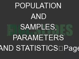
Populations vs. Sample

A

population

includes each element from the set of observations that can be made.A sample consists only of observations drawn from the population.

population

sample

Inferential

Statistics

Exploratory Data Analysis

samplingSlide3

Characteristic of

a

population

vs. characteristic

of

a sample

A a measurable characteristic of a population, such as a mean or standard deviation, is called a 

parameter, but a measurable characteristic of a sample is called a 

statistic.

Population

Expect

ed

value

(mean), resp. Medianx0,5Variance (dispersion), resp. Std. deviationσProbabilityπSampleSample mean (average)Sample medianSample varianceS2Sample std. deviationSRelative frequencyp

Population

Median

x

0,5

Std

.

deviation

σ

Probability

π

Sample

Sample variance

S

2

Sample

std

.

deviation

S

Relative

frequency

pSlide4

Sampling Distributions

A sampling distribution is created by, as the name suggests,

sampling

. The method we will employ on the rules of probability

and the laws of expected value and variance to derive the sampling distribution.

For example, consider the roll of one and two dice

s…Slide5

A fair die

is thrown infinitely many times,

with the random variable = # of spots on any throw.The probability distribution of

is:

T

he mean

, variance and standard deviation are calculated as:

,

1

2

3

456

1/6

1/6

1/6

1/6

1/6

1/6

1234561/61/61/61/61/61/6

The roll of one dieSlide6

A sampling distribution is created by looking at all samples of size n=2 (i.e. two dice) and their means

.

The

roll

of Two Dice

s

The

Sampling Distribution of

Mean

Sample

Mean

Sample

MeanSampleMean{1, 1}1,0{3, 1}2,0{5, 1}3,0{1, 2}1,5{3, 2}2,5{5, 2}3,5{1, 3}2,0{3, 3}3,0{5, 3}4,0{1, 4}2,5{3, 4}3,5{5, 4}4,5{1, 5}3,0{3, 5}

4,0

{

5

,

5}

5,0{1, 6}3,5{3, 6}4,5{5, 6}5,5{2, 1}1,5{4, 1}2,5{6, 1}

3,5{2, 2}2,0{4, 2}3,0{6, 2}4,0{2, 3}2,5{4, 3}3,5{6, 3}4,5{2, 4}3,0{4, 4}4,0{6, 4}5,0{2, 5}3,5{4, 5}4,5{6, 5}5,5{2, 6}4,0{4, 6}5,0{6, 6}6,0Slide7

A sampling distribution is created by looking at all samples of size

n

=2 (i.e. two dice) and their means

.

While there are 36 possible samples of size 2, there are only 11 values for

, and some (e.g.

) occur more frequently than others (e.g.

).

The

roll

of Two Dice

s

The Sampling Distribution of Mean1,01/361,52/362,03/362,54/363,05/363,56/36

4,0

5/36

4,5

4/36

5,0

3/365,5

2/366,01/361,01/361,52/362,03/362,54/363,05/363,56/36

4,0

5/364,54/365,03/365,52/366,0

1/36Slide8

A sampling distribution is created by looking at

all samples of size

n

=2 (i.e. two dice) and their means.

,

The

roll

of Two Dice

s

The

Sampling Distribution of Mean1,01/361,5

2/36

2,0

3/36

2,5

4/36

3,05/36

3,56/364,05/364,54/365,03/365,52/366,01/361,01/36

1,5

2/362,03/362,54/363,05/363,5

6/364,05/364,54/365,03/36

5,5

2/36

6,0

1/36Slide9

A sampling distribution is created by looking at

all samples of size

n

=2 (i.e. two dice) and their means.

= # of spots on

i-

th

dice

,

,

The

roll of Two DicesThe Sampling Distribution of Mean1,0

1/36

1,5

2/36

2,0

3/36

2,54/36

3,05/363,56/364,05/364,54/365,03/365,52/366,01/36

1,0

1/361,52/362,03/362,54/363,0

5/363,56/364,05/364,54/36

5,0

3/36

5,5

2/36

6,0

1/36Slide10

Compare

= # of spots on

i-

th

dice

, ,

Note

that

:

,

Distribution of XSampling Distribution of  Slide11

Generalize - Central Limit

Theor

em

The sampling distribution of the mean of a random sample drawn from any population is

approximately normal for a

sufficiently large sample size.

,

,

The larger the sample size, the more closely the sampling distribution of

X

will resemble a normal distribution.

 Slide12

Central Limit Theorem

…

random

variable,

,

Note

that

:

,

, … standard error Same Distribution of all  Sampling Distribution of    Slide13

Generalize - Central Limit

Theor

em

The sampling distribution of

drawn from any population is approximately normal for a

sufficiently large sample size.

In many practical situations, a

sample size of 30

may

be sufficiently large to allow us to use the normal distribution as an approximation for the sampling distribution of

.

Note: If

is normal, is normal. We don’t need Central Limit Theorem in this case.  Slide14

The foreman of a bottling plant has observed that the amount of soda in each “32-ounce” bottle is actually a normally distributed random variable, with a mean of 32

,

2

ounces and a standard deviation of 0,3 ounce.A) If a customer buys one bottle, what is the probability that the bottle will contain more than 32 ounces?Slide15

The foreman of a bottling plant has observed that the amount of soda in each “32-ounce” bottle is actually a normally distributed random variable, with a mean of 32

,

2

ounces and a standard deviation of 0,3 ounce.B) If a customer buys a carton of four bottles, what is the probability that the mean amount of the four bottles

will be greater than 32 ounces?Slide16

Graphically Speakin

g

W

hat

is the probability that one bottle will contain more than 32 ounces?

W

hat

is the probability that the mean of four bottles will exceed 32

oz

?

 Slide17

The probability distribution of 6-month incomes of account executives has mean $20,000 and standard deviation $5,000.

A

)

A single executive’s income is $20,000. Can it be said that this executive’s income exceeds 50% of all account executive incomes?Answer: No information given about shape of distribution of X; we do not know the median of 6-mo

nth incomes.Slide18

The probability distribution of 6-month incomes of account executives has mean $20,000 and standard deviation $5,000.

B

)

=64 account executives are randomly selected. What is the probability that the sample mean exceeds $20,500?

 Slide19

A sample of size

=16 is drawn from a normally distributed population with

and

. Find

(

Do we need the Central Limit Theorem to solve

?)

 Slide20

Battery life

. Guarantee: avg. battery life in a case of 24 exceeds 16 hrs. Find the probability that a randomly selected case meets the guarantee.

 Slide21

Cans of salmon are supposed to have a net weight of 6 oz. The producer says that the net weight is a random variable with mean

=

6

,05 oz. and stand. dev. =0,18 oz.

Suppose

you take a random sample of 36 cans and calculate the sample mean weight to be 5.97 oz.

Find the probability that the mean weight of the sample is less than or equal to 5.97 oz.

Since

, either

you observed a “rare” event (recall: 5,

97

oz

is

2,67 stand. dev. below the mean) and the mean fill is in fact 6,05 oz. (the value claimed by the producer), the true mean fill is less than 6,05 oz (the producer is lying ). Slide22

Sampling Distribution of a Proportion

The estimator of a population proportion

of successes is the

sample proportion . That is, we count the number of successes in a sample and compute:

X

is the number of successes,

n

is the sample size.

 Slide23

Normal Approximation to Binomial

Binomial distribution with

n

=20 and with a normal approximation superimposed (

and

)

.

 Slide24

Normal Approximation to Binomial

Normal approximation to the binomial works best when the number of experiments

(sample size) is large, and the probability of success

is close to 0

,5.

For the approximation to provide good results one condition should be met:

.

 Slide25

Sampling Distribution of a Sample Proportion

Using the laws of expected value and variance, we can determine the mean, variance, and standard deviation of

.

,

,

Sample proportions can be standardized to a standard normal distribution using this formulation:

.

standard error of the proportionSlide26

Find the probability that of the next 120 births, no more than 40% will be boys. Assume equal probabilities for the births of boys and girls.Slide27

12% of students at NCSU are left-handed. What is the probability that in a sample of 50 students, the sample proportion that are left-handed is less than 11%?Slide28

Sampling Distribution: Difference of two means

Assumption

:

Independent random samples be drawn from each of two normal populations

.

If this condition is met, then the sampling distribution of the

difference between the two sample means will be normally distributed if the populations are both normal.

Note: I

f the two populations are not both normally distributed, but the sample sizes are “large” (>30), the distribution of

is

approximately

normal – Central Limit Theorem

.

 Slide29

Sampling Distribution: Difference of two means

,

standard

error

of

the

difference

between two meansSlide30

Sampling Distribution: Difference of two proportions

Assumption:

Central Limit Theorem

:

,

 Slide31

Sampling Distribution: Difference of two means

,

standard

error

of

the

difference

between

two

proportionsSlide32

Special Continous

DistributionSlide33

, pak

Distribution

Degrees

of

Freedom

Using

of

Distribution Slide34

The Acme Battery Company has developed a new cell phone battery. On average, the battery lasts 60 minutes on a single charge. The standard deviation is 4 minutes.Suppose the manufacturing department runs a quality control test. They randomly select 7 batteries.

What

is probability, that the standard deviation of the selected batteries is greather than 6 minutes?Slide35

Student's t Distribution

,

and

are independent

variables

If

,

then

has Student‘s t Distribution with  degrees of freedom, .Using of Student‘s tDistributionThe t distribution should be used with small samples from populations that are not approximately normal. Slide36

Acme Corporation manufactures light bulbs. The CEO claims that an average Acme light bulb lasts 300 days. A researcher randomly selects 15 bulbs for testing. The sampled bulbs last an average of 290 days, with a standard deviation of 50 days. If the CEO's claim were true, what is the probability that 15 randomly selected bulbs would have an average life of no more than 290 days?Slide37

F Distribution

The f Statistic

The 

f statistic, also known as an f value, is a random variable that has an F distribution.

Here are the steps required to compute an f

 statistic:Select a random sample of size n

1 from a normal population, having a standard deviation equal to σ1.Select an independent random sample of size 

n2 from a normal population, having a standard deviation equal to σ2.

The f statistic is the ratio of s12/σ12 and s22

/σ22.Slide38

F Distribution

Here

are the steps required to compute an 

f statistic:Select a random sample of size n1 from a normal population, having a standard deviation equal to σ

1.

Select an independent random sample of size n2 from a normal population, having a standard deviation equal to σ

2.The f statistic is the ratio of s

12/σ12 and s

22/σ22.

Degrees

of

freedomSlide39

Suppose

you

randomly

select

7

women

from a population

of

women

, and 12 men from a population of men. The table below shows the standard deviation in each sample and in each population. Find probability, that sample standard deviation of men is greather than twice sample standard deviation of women.PopulationPopulation standard deviationSample standard deviationWomen3035

Men

50

45Slide40

Study materials :

http://homel.vsb.cz/~bri10/Teaching/Bris%20Prob%20&%20Stat.pdf

(p. 93 - p.104)

http://stattrek.com/tutorials/statistics-tutorial.aspx?Tutorial=Stat

(Distributions – Continous (Students

,

F Distribution) + Estimation